1.1 Functions
1.1 Functions
What is a function?
The natural world is full of relationships between quantities that change. When we see these relationships, it is natural for us to ask: If I know one quantity, can I then determine the other? This establishes the idea of an input quantity, or the independent variable, and a corresponding output quantity, or the dependent variable. From this we get the notion of a functional relationship in which the output can be determined from the input.
Concept Check
Can you determine what is input and what is output in a relationship? Which value in a relationship represents the independent and which represents the dependent variable? Try this quick set of multiple choice exercises:
MathMatize: Independent vs. dependent variables
For some quantities, like height and age, there are certainly relationships between these quantities. Given a specific person and any age, it is easy enough to determine their height, but if we tried to reverse that relationship and determine height from a given age, that would be problematic since most people maintain the same height for many years.
In this course we will be working with relationships of the first type, where for each input value we get one and only one output value. In other words, there is no ambiguity about the result - it is uniquely determined by the given information, or the input. These types of relationships are called functions and have many very useful properties that will allow us to study those relationships in great detail.
Function
A function, in a mathematical sense, is rule for a relationship between an input (independent) quantity and an output (dependent) quantity in which each input value uniquely determines one output value. We say that "the output is a function of the input."

Example 1
Is height of a person a function of their age? Is age of a person a function of their height?
Answer: To determine if one quantity is a function of another, we have to determine if there is a rule that can determine a quantity given another quantity in a unique, unambiguous way. In other words, this rule cannot give us two or more possible outcomes for a single input quantity.
In the height and age example above, it would be correct to say that the person's height is a function of their age since each age uniquely determines a height. In other words, at any point in their life, a person has one and only one height. For example, on my 18th birthday I had exactly one height of 69 inches.
However, age is not a function of height since one height input might produce more than one output age. For example, for an input height of 70 inches, there is more than one output of age since I was 70 inches at the age of 20 and 21.
Concept Check
Can you determine if a relationship could be represented as a function or possibly not? Test your understanding of the concept of function through these quick multiple choice and fill-in-the-blank exercises:
MathMatize: Function or not?
The language minefield: Note that the word "function" is used in different contexts with different meanings. In colloquial, every day use, it can represent a notion of one thing dependent on another but without the precision of a rule. For example, we may say "how much I learn is a function of how much I practice", meaning that the amount learned is dependent on the amount of practice, but here there is no inherent rule associated with that relationship saying exactly how much is learned given how much practice is completed. Another example is the use of the term "function" in coding, where a function is defined as a self-contained module of code that accomplishes a particular task. Here again there is a dependence relationship represented through a set of initial parameters representing the input and a task that uses assigned values of those parameters to produce an output, though output in this case may be a collection of values. When using the word "function" in this course, we will be using the definition shared above within its mathematical sense, and also presented more formally in the text that follows.
Function Notation
As you can see from the Concept Check exercises above, talking about relationships can get quite "wordy". To simplify writing out expressions and equations involving functions, a simplified notation is often used. We also use descriptive variables to help us remember the meaning of the variables used in the problem.
Recall that a function is rule for a relationship between an input (independent) quantity and an output (dependent) quantity in which each input value uniquely determines one output value. We say that "the output is a function of the input."
More formally, a function is a rule that assigns to each element in a set [latex]D[/latex] exactly one element in a set [latex]E[/latex].
Sometimes a function is referred to as a map or a mapping.
If the name of a function is [latex]f[/latex], we write [latex]f:D\to E[/latex] and we read this as [latex]"f[/latex] is a function from [latex]D[/latex] to [latex]E".[/latex]
We call the set [latex]D[/latex] the domain of [latex]f[/latex] and the set [latex]E[/latex] the codomain of [latex]f[/latex].
The domain is the set of all input values of the function that produce an output. The set of all output values of a function is called the range of the function and is a subset of the codomain.
The language minefield: Note that we are using in the definition of a function the word set which can colloquially have many different meanings (a volleyball set, a set of exercises, the cake did not set, to set a grade etc.). In math, the word set has a specific meaning - it represents a collection of objects. These objects can be number values, names, physical objects, characteristics etc.
In mathematics, we classify numbers using set definitions, such as the real number set, denoted by [latex]\mathbb{R}[/latex], the set of integers [latex]\mathbb{Z}[/latex], the set of natural numbers [latex]\mathbb{N}[/latex], the set of rational numbers [latex]\mathbb{Q}[/latex], etc.
If you are familiar with coding using programming languages, you may be familiar with sets represented through:
- numeric data types such as NUMBER, INT, INTEGER, BIGINT, SMALLINT, TINYINT, BYTEINT, FLOAT, FLOAT4, FLOAT8, etc.
- string and binary data types such as VARCHAR, CHAR, STRING, BINARY, etc.
- logical data type BOOLEAN
- date and time data types such as DATE, DATETIME, TIME, TIMESTAMP, etc.
- ... and others
Function Notation
If the variable [latex]f[/latex] represents the output variable of a function and [latex]x[/latex] represents the input variable of that function, then we use the notation [latex]f(x)[/latex] to represent this relationship and we read it as "[latex]f[/latex] of [latex]x[/latex]".
Depending on the context, [latex]f(x)[/latex] may mean one of the two things:
- [latex]f(x)[/latex] is a function [latex]f[/latex] of [latex]x[/latex]
- [latex]f(x)[/latex] is the value of [latex]f[/latex] at [latex]x[/latex]
It is common to refer to a function in general using [latex]f[/latex] and [latex]x[/latex] but the relationship between them is only implied through the function notation. For example, [latex]x(f)[/latex] would imply that [latex]x[/latex] is a function of [latex]f[/latex] and so that in this relationship the output is [latex]x[/latex] and it is uniquely determined by the input [latex]f[/latex].
Using the example of age and height above, rather than write "height is a function of age", we could use the descriptive variable [latex]h[/latex] to represent height and we could use the descriptive variable [latex]a[/latex] to represent age. We can then simply write [latex]h(a)[/latex] to say "height is a function of age".
Remember that we can use any variable to name the function; the notation [latex]h(a)[/latex] shows us that [latex]h[/latex] depends on [latex]a.[/latex] The value [latex]a[/latex] must be put into the function [latex]h[/latex] to get a result. Be careful - the parentheses indicate that age is the input for the function (note: do not confuse these parentheses with multiplication!).
Example 2
A function [latex]N(y)[/latex] gives the number of police officers, [latex]N[/latex], in a town in year [latex]y[/latex]. What does [latex]N(2005) = 300[/latex] tell us?
Answer: When we read [latex]N(2005)=300[/latex] (or "N at 2005 is 300"), we see the input quantity is 2005 and the output quantity is 300. In [latex]N(y)[/latex] the input represents the year [latex]y[/latex] and the output represents the number of police officers [latex]N[/latex]. Therefore, [latex]N(2005)=300[/latex] tells us that in the year 2005 there were 300 police officers in the town.
Concept Check
Function notation can be confusing. Check if you are on the right track connecting words to symbols and symbols to words when discussing relationships represented through functions:
Try MathMatize: Function Notation
Representations of Functions
Functions can be represented in many ways: words or diagrams (as we did in the last few examples), tables of values, graphs or formulas.
Functions represented through tables
Represented as a table, we are presented with a list of input and output values. By convention, the first row (or column) in a table represents the independent variable.
For example, the table below represents the age of children in years and their corresponding heights. While some tables show all the information we know about a function, this particular table represents just some of the data available for height and ages of children.
| [latex]a[/latex], age in years | 4 | 5 | 6 | 7 | 8 | 9 | 10 |
| [latex]h[/latex], height in inches | 40 | 42 | 44 | 47 | 50 | 52 | 54 |
In the above example, the independent variable (or the input) is the age of a child, measured in years and denoted by [latex]a[/latex], because the first row, by convention, represents the independent variable. The dependent variable (or the output) is the height of the child, denoted by [latex]h[/latex] and measured in inches. The notation for this function would be [latex]h(a)[/latex].
Another example of a function represented through a data table is the following example of a relationship between app run time and the number of nodes in the network:
| Number of nodes ([latex]n[/latex]) | Run time – seconds ([latex]t[/latex]) |
| 200 | 29 |
| 500 | 58 |
| 1000 | 175 |
| 1500 | 729 |
| 2000 | 1458 |
| 2500 | 2479 |
| 3000 | 4375 |
| 4000 | 12250 |
Note that, in the above example the independent variable is the number of nodes, denoted by [latex]n[/latex], because the first column is, by convention, the independent variable (or the input). The dependent variable (or the output) is the run time, denoted by [latex]t[/latex] and measured in seconds. The notation for this function would be [latex]t(n)[/latex].
Example 3
Which of these tables defines a function (if any)?
| a) | Input | Output | b) | Input | Output | c) | Input | Output | ||
| 2 | 1 | -3 | 5 | 1 | 0 | |||||
| 13 | 13 | 0 | 1 | 5 | 2 | |||||
| 8 | 6 | 4 | 5 | 5 | 4 | |||||
Answer: Tables a) and b) define functions. In both, each input corresponds to exactly one output. Table c) does not define a function since the input value of 5 corresponds to two different output values.
Concept Check
Here are some examples relationships represented using tables. Which ones of them represent functions?
MathMatize: Functions from data tables
Functions represented through graphs
Often a graph of a relationship can be used to represent a function and, conversely, a function could be represented by a graph. By convention, graphs are typically created with the input quantity along the horizontal axis and the output quantity along the vertical. As such, a point on the graph of a function can be viewed through coordinates [latex](input, output)[/latex] and a graph represents a function only if there is no point on the graph that for the same value on the horizontal axis produces two or more values on the vertical axis.
Example 4
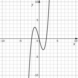
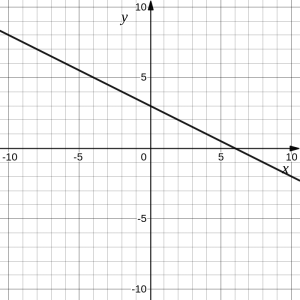
Which of these graphs represents a function?
 |
 |
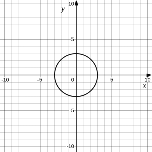 |
Answer: Looking at the three graphs above, the first two represent a function [latex]y(x)[/latex] since for each input value [latex]x[/latex]along the horizontal axis there is exactly one corresponding output value, determined by the [latex]y[/latex]-value of the graph. The third graph does not define a function [latex]y(x)[/latex] since some input values, such as [latex]x=2[/latex], correspond with more than one output value.
Vertical Line Test
Reading Graphs of Functions
Reading a function using its graph requires taking the given input (horizontal axis) and using the graph to look up the corresponding output (vertical axis). Conversely, we can use the graph by taking a given output (vertical axis) and looking at the graph to determine the corresponding input(s) (horizontal axis).
Example 5
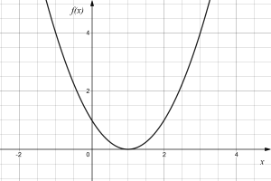 Consider the graph to the right.
a) Evaluate [latex]f(2)[/latex].
b) Solve [latex]f(x)=4[/latex].
Answer:
a) To evaluate [latex]f(2)[/latex], we find the input of [latex]x=2[/latex] on the horizontal axis. Moving up to the graph gives the point [latex](2, 1)[/latex], giving an output of [latex]f(x)=1[/latex]. So [latex]f(2)=1[/latex].
b) To solve [latex]f(x)=4[/latex], we find the value [latex]4[/latex] on the vertical axis because if [latex]f(x)=4[/latex] then [latex]4[/latex] is the output. Moving horizontally across the graph gives two points with the output of [latex]4[/latex]: [latex](-1,4)[/latex] and [latex](3,4)[/latex]. These give the two solutions to [latex]f(x)=4[/latex]: [latex]x=-1[/latex] or [latex]x=3[/latex]. This means [latex]f(-1)=4[/latex] and [latex]f(3)=4[/latex], or when the input is [latex]-1[/latex] or [latex]3[/latex], the output is [latex]4[/latex].
Note that while the graph in the previous example is a function, getting two input values for the output value of 4 shows us that this function is not one-to-one, i.e., there are two or more inputs that map to the same output. This, in turn, means this relationship cannot be reversed, i.e., [latex]f[/latex] is a function of [latex]x[/latex], but [latex]x[/latex] is not a function of [latex]f[/latex] because otherwise there would be input values [latex]f[/latex] giving more than one output [latex]x[/latex]. On the other hand, if a function is one-to-one, i.e., no output values are repeated, then the function is invertible.
Functions represented through formulas
When possible, it is very convenient to represent function relationships using formulas. If it is possible to express the output as a formula involving the input quantity, then this formula represents the rule of that function.
Example 6
Express the relationship [latex]2n+6p=12[/latex] as a function [latex]p(n)[/latex], if possible.
Answer:
To express the relationship [latex]p(n)[/latex], we need to be able to write the relationship where [latex]p[/latex] is a function of [latex]n[/latex], which means being able to determine [latex]p[/latex] using [latex]n[/latex], or writing this relationship as
[latex]p=\text{something involving }n[/latex]
So, using the given equation, we have
[latex]\begin{align*}&2n+6p=12\\&\Rightarrow 6p=12-2n\\&\Rightarrow p=\frac{12-2n}{6}=\frac{12}{6}-\frac{2n}{6}=2-\frac{1}{3}n \end{align*}[/latex]
Having rewritten the formula to solve for [latex]p[/latex], we can now express [latex]p[/latex] as a function of [latex]n[/latex]:
[latex]p(n)=2-\frac{1}{3}n[/latex]
Note that not every relationship can be expressed as a function with a formula.
Evaluating Functions
When we work with functions, there are typically two things we do: solving for the output and solving for the input.
Solving for the output, also referred to as evaluating a function, is what we do when we know an input, and we use the function to determine the corresponding output. Evaluating will always produce one result because each input of a function corresponds to exactly one output.
Solving for the input involving a function is what we do when we know an output, and we reverse the rule of the function to determine the inputs that would produce that output. Solving for the input of a function could produce more than one solution since different inputs can produce the same output.
Example 7
Use the table shown for [latex]g(n)[/latex]
| [latex]n[/latex] | 1 | 2 | 3 | 4 | 5 |
| [latex]g[/latex] | 8 | 6 | 7 | 6 | 8 |
a) Evaluate [latex]g(3)[/latex].
b) Solve [latex]g(n)=6[/latex].
Answer:
a) Evaluate [latex]g(3)[/latex]: Evaluating [latex]g(3)[/latex] (read: g of 3) means that we need to determine the output value, [latex]g[/latex] given the input value of [latex]n=3[/latex]. Looking at the table, we see the output corresponding to [latex]n=3[/latex] is [latex]g=7[/latex], allowing us to conclude [latex]g(3) = 7[/latex].
b) Solve [latex]g(n)=6[/latex]: Solving [latex]g(n)=6[/latex] means we need to determine which input values, [latex]n[/latex], produce an output value of 6. Looking at the table we see there are two solutions: [latex]n = 2[/latex] and [latex]n = 4[/latex] because both producethe output is [latex]g=6[/latex] and they are the only input values that produce this output.
As with tables and graphs, it is common to solve for inputs and outputs with functions involving formulas. Solving for the output will then require replacing the input variable in the formula with the value provided and calculating the value of the expression. Solving for the input will require replacing the output variable in the formula with the value provided, and rearranging the function formula to solve for the input(s) that would produce that output.
Example 8
Given the function [latex]k(t)=t^3+2[/latex]:
a) Evaluate [latex]k(2)[/latex].
b) Solve [latex]k(t)=1[/latex].
Answer:
a) To evaluate [latex]k(2)[/latex], we substitute the input value 2 into the formula wherever we see the input variable [latex]t[/latex], then simplify:
[latex]k(2) = 2^3+2 = 8+2 =10[/latex]
So [latex]k(2)=10[/latex].
b) To solve [latex]k(t)=1[/latex], we set the formula for [latex]k(t)[/latex] equal to 1, and solve for the input value that will produce that output. Recall that solving an equation involves identifying the unknown variable ([latex]t[/latex]), analyzing the operations taking place on the variable and their order (first raise to exponent of three, then add 2), and finally applying to both sides of the equation the opposite operations, in the opposite order (first subtract two, then take the third root):
[latex]\begin{align*} k(t)&=1&\\ &\Rightarrow t^3+2=1&\text{substitute the original formula}\\ &\Rightarrow t^3=-1&\text{subtract 2 from each side}\\ &\Rightarrow t=-1&\text{take the cube root of each side} \end{align*}[/latex]
Note: When solving for the input using formulas, you can check your answer by using your solution in the formula of the function to see if your calculated answer is correct. For example, we want to verify if [latex]k(t)=1[/latex] is true when [latex]t=-1[/latex]:
[latex]\begin{align*}k(-1)&=(-1)^3+2\\&=-1+2\\& = 1\end{align*}[/latex]
which was the desired result.
Basic Function Types
There are some basic functions that one should know and be able to recognize through name and shape. General functions will often come from these basic types through various operations and transformations. These basic types are listed below and for their definitions we will use [latex]x[/latex] as the input variable and [latex]f(x)[/latex] as the output variable.
Basic functions
Here are some of the most common functions. We will discuss others in the sections that follow.
| Constant: | [latex]f(x)=c[/latex], where [latex]c[/latex] is a constant (number) |
| Identity: | [latex]f(x)=x[/latex] |
| Absolute Value: | [latex]f(x)=|x|[/latex] |
| Quadratic: | [latex]f(x)=x^2[/latex] |
| Cubic: | [latex]f(x)=x^3[/latex] |
| Reciprocal: | [latex]f(x)=\frac{1}{x}[/latex] |
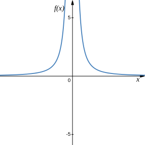
| General reciprocal: | [latex]f(x)=\frac{1}{x^2}[/latex] |
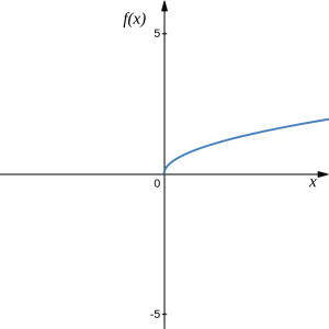
| Square root: | [latex]f(x)=\sqrt[2]{x}=\sqrt{x}[/latex] |
| Cube root: | [latex]f(x)=\sqrt[3]{x}[/latex] |
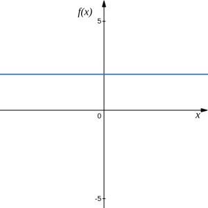
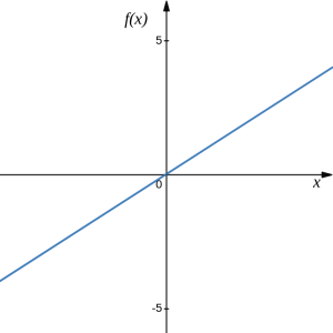
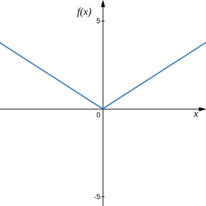
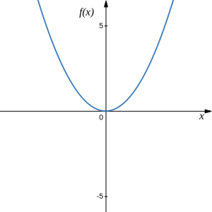
Below are the graphs of these functions:
 |
 |
 |
| Constant function, [latex]f(x)=c[/latex] ([latex]c[/latex] is 2 in this picture). |
Identity function: [latex]f(x)=x[/latex]. | Absolute Value function: [latex]f(x)=|x|[/latex] |
 |
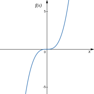 |
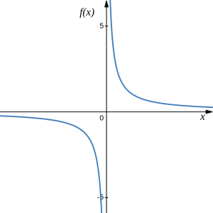 |
| Quadratic function: [latex]f(x)=x^2[/latex] | Cubic function: [latex]f(x)=x^3[/latex] | Reciprocal function: [latex]f(x)=\frac{1}{x}[/latex] |
 |
 |
 |
| Reciprocal squared: [latex]f(x)=\frac{1}{x^2}[/latex] | Square root: [latex]f(x)=\sqrt[2]{x}=\sqrt{x}[/latex] | Cube root: [latex]f(x)=\sqrt[3]{x}[/latex] |
Visualization
See these functions for yourself:
Geogebra: Basic types of functions (click on circle beside the function whose graph you would like to explore)
Domain and Range
One of our main goals in mathematics is to model the real world with mathematical functions. In doing so, it is important to keep in mind the limitations of those models we create. In other words, since a function is represented by a rule, we must know when this rule can be applied, i.e., the domain of the function. It is also often helpful to know what possible results this function can produce, which is the range of the function. Recall that:
Range of a function is the set of all possible output values of the function.
We know what we mean by the words function, set, input, and output, but what do we mean here by the word possible?
When we are speaking of the possible input values, we mean all input values that produce an output value in the relationship represented through the given function. So the domain of a function is all input values that produce and output, or all possible inputs for short.
When we are speaking of the possible output values, we mean all output values that are produced by some input value. So the range of a function is completely determined by the possible input values, or the domain of the function, and the rule that describes the function, through which the outputs are produced.
Therefore, both the domain and the range are determined through the investigation of input values that are allowed to be used in the function, both rule-wise (or mathematically), and contextually.
Let's first consider the domain of a function defined by a formula, without a specific context in mind.
Domain of a function given through a formula
In general, if our input values are numbers and our function is represented through a formula, then the output values are the results of a calculation. Hence we would have to make sure that the number used as the input will not "break" the calculation. In other words, we have to make sure that the formula calculation steps can be performed using that input number. Therefore, to determine the domain of a function mathematically, or its so-called natural domain, we have to determine all possible numerical values that can be used in the formula to produce a result.
How do we do this?
First, we note that a formula is just a series of calculations performed using the variable(s) given. There are two aspects we have to consider. In general, to produce an output given an input, we will have to perform actions in a prescribed order.
In a formula, the actions involved are typically mathematical operations such as addition, subtraction, multiplication, addition etc. There are others as well, and we'll discuss them in the next section of this chapter. We use symbols and conventions about symbol use (and non-use) to denote mathematical operations and we use certain nomenclature to describe the results of those operations. For example:
sum is the result of addition, denoted by the symbol [latex]+[/latex]
difference is the result of subtraction, denoted by the symbol [latex]-[/latex]
product is the result of multiplication, denoted by the symbol [latex]\cdot[/latex] (or [latex]\times[/latex])
quotient is the result of division, denoted by the fraction symbol [latex]\frac{\ }{\ }[/latex] (or [latex]\div[/latex])
By convention, when an operation symbol is omitted between two numerical values, it is generally assumed the operation is multiplication. However, there is an exception to this when we write a number followed by a fraction, in which case the absence of the operation symbol means addition. For example:
[latex]2x[/latex] means the product of [latex]2[/latex] and the value of [latex]x[/latex]
(read as "two [latex]x[/latex]" or, when clarity is required, "two times [latex]x[/latex]")
[latex]xy[/latex] means the product of the value of [latex]x[/latex] and the value of [latex]y[/latex]
(read as "[latex]xy[/latex]" or, when clarity is required, "[latex]x[/latex] times [latex]y[/latex]")
[latex]2(x+y)[/latex] means the product of [latex]2[/latex] and the sum of the values of [latex]x[/latex] and [latex]y[/latex]
(read, with appropriate pausing, as "two times pause [latex]x[/latex] plus [latex]y[/latex]")
[latex]2 \frac{x}{y}[/latex] means the sum of [latex]2[/latex] and the quotient of [latex]x[/latex] and [latex]y[/latex]
(read, with appropriate pausing, as "two and pause [latex]x[/latex] over [latex]y[/latex]" or, when clarity is required, "two plus pause [latex]x[/latex] divided by [latex]y[/latex]")
[latex]k \dfrac{x}{y}[/latex] means the sum of the value of [latex]k[/latex] and the quotient of [latex]x[/latex] and [latex]y[/latex]
(read, with appropriate pausing, as "[latex]k[/latex] and pause [latex]x[/latex] over [latex]y[/latex]" or, when clarity is required, "[latex]k[/latex] plus pause [latex]x[/latex] divided by [latex]y[/latex]")
In addition, the order of mathematical operations is set by well-established conventions. For example, recall that, unless directed otherwise through the use of parentheses, exponents are performed before multiplication and division, and multiplication and division are performed before addition and subtraction.
So, to determine the domain of a function defined through a formula, we must identify which values for the input variable can produce an output value, and so we must first analyze two things: which operations are taking place on the input variable, and in which order. Then we have to consider, for each of the operations, the conditions under which the value of the input variable will yield a result. Finally, we then consolidate all of the conditions to determine which input values satisfy all of the conditions. This consolidation then describes the totality of all possible input values, i.e., the domain of the function.
In determining these conditions dictated by the operations, we remind ourselves that, when dealing with real numbers:
Any two numbers can be added, so there is no restriction in addition, i.e., [latex]a+b\ \checkmark[/latex]
Any two numbers can be subtracted, so there is no restriction in subtraction, i.e., [latex]a-b\ \checkmark[/latex]
Any two numbers can be multiplied, so there is no restriction in multiplication, i.e., [latex]a\cdot b\ \checkmark[/latex]
Any two numbers can be divided, as long as the divisor (the number we are dividing by) is not zero, i.e., the denominator of a fraction must not equal to zero.
Any non-negative number can be raised to any exponent, except zero raised to the power of zero, which is undefined, i.e., [latex]0^0[/latex] is undefined, otherwise [latex]b^a\ \checkmark[/latex] if [latex]b\ge 0[/latex].
Any number, including a negative number, can be raised to any exponent if the exponent can be written as a simplified fraction whose denominator is an odd number. In particular, an odd root of any number has a value, so there is no restriction in calculating an odd root.
Only non-negative numbers can be raised to an exponent if the exponent can be written as a simplified fraction whose denominator is an even number. In particular, an even root of a number has a value only if that number is not negative.
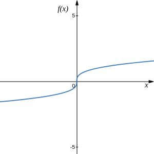
For example, consider the function
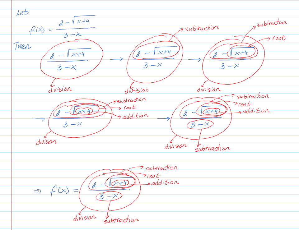
[latex]f(x)=\dfrac{2-\sqrt{x+4}}{3-x}[/latex]
Talking ourselves through the operations taking place in the formula, we can see that the output is a quotient of two values: the numerator and the denominator of the fraction. Therefore, there is division, where the numerator is a difference between a value and the root of a sum of two values, and the denominator is a difference of two values.
Visually, we can describe this analysis process as follows:
Therefore, since addition and subtraction have no restriction, only the division and the root are potentially problematic. Since the root is the second root (remember that [latex]\sqrt{\#}[/latex] means [latex]\sqrt[2]{\#}[/latex]), we'll have to make sure that what is under the root is not negative, and we'll also have to make sure that the denominator in the division is not equal to zero. Visually:
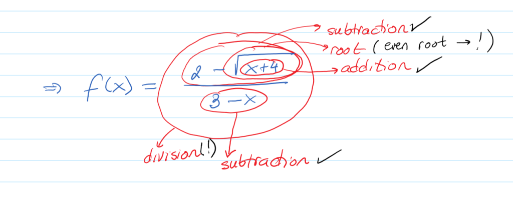
Therefore, we have two and only two conditions on [latex]x[/latex]:
[latex]x+4\ge 0\Rightarrow x\ge -4[/latex]
[latex]3-x\neq 0\Rightarrow x\neq 3[/latex]
So, for [latex]f(x)[/latex] to be defined (or calculable), [latex]x\ge -4[/latex] and [latex]x\neq 3[/latex], i.e.,
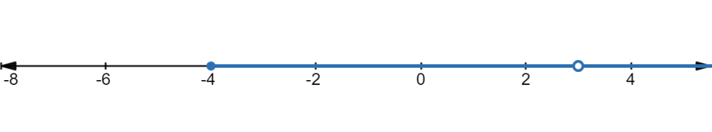
Therefore, the domain of [latex]f(x)[/latex] is [latex]\{x\in \mathbb{R}\vert x\ge -4, x\neq 3\}[/latex] or, written in interval form, [latex][-4, 3)\cup(3,\infty)[/latex].
As can be seen from above example, interval notation is a more compact alternative to the set notation using inequalities. In the interval notation, the possible values are bounded by the starting and ending values. Curved parentheses are used for strictly less than (or strictly more than), and square brackets are used for less than or equal to (or more than or equal to) a specified value. Since infinity is not a number, we can’t include it in the interval, and so we always use curved parentheses with [latex]\infty[/latex] and [latex]-\infty[/latex]. The curved parentheses are also referred to as open while the square ones are referred to as closed. The table below will help you see how inequalities correspond to interval notation:
| Inequality | Interval Notation |
| [latex]5\lt h\leq 10[/latex] | [latex](5, 10][/latex] |
| [latex]5 \lt h \lt 10[/latex] | [latex](5, 10)[/latex] |
| [latex]5\leq h \lt10[/latex] | [latex][5, 10)[/latex] |
| [latex]h \lt10[/latex] | [latex](-\infty,10)[/latex] |
| [latex]h\geq10[/latex] | [latex][10,\infty)[/latex] |
| All real numbers ([latex]\mathbb{R}[/latex]) | [latex](-\infty,\infty)[/latex] |
The language minefield: Note that, in mathematics, parentheses symbols are used in many different ways and the only way to interpret them correctly is to take into account the context within which they are used. For example,
[latex](a+b)[/latex] means "first calculate the sum of [latex]a[/latex] and [latex]b[/latex]".
[latex](a,b)[/latex] could represent an interval, in which case it means "all values that are greater than [latex]a[/latex] and less than [latex]b[/latex]" or "all values between [latex]a[/latex] and [latex]b[/latex], not including either".
[latex](a,b)[/latex] could represent coordinates of a point on a graph, where [latex]a[/latex] represents the corresponding value on the horizontal axis and [latex]b[/latex] represents the corresponding value on the vertical axis.
[latex](a,b)[/latex] could represent a specific data point of a function, where [latex]a[/latex] represents the value of the input (or the independent variable) and [latex]b[/latex] represents the corresponding value of the output (or the dependent variable).
Example 9
Describe the intervals of values shown on the line graph below using set and interval notations:
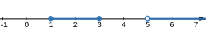
Answer:
To describe the values of [latex]x[/latex] that lie in the intervals shown above we would say: [latex]x[/latex] is a real number greater than or equal to 1 and less than or equal to 3, or a real number greater than 5.
Written as an inequality, it is [latex]1\leq x\leq 3[/latex] or [latex]x \gt 5[/latex].
Written in interval notation, it is [latex][1,3]\cup(5,\infty)[/latex].
Example 10
Find the domain of each function:
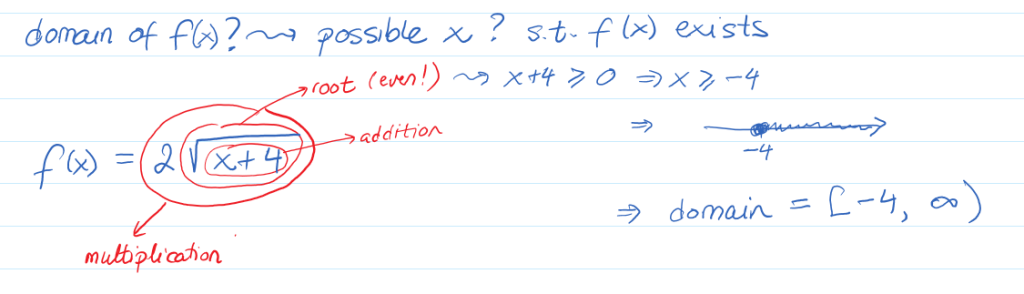
a) [latex]f(x)=2\sqrt{x+4}[/latex]
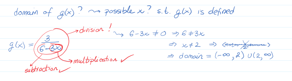
b) [latex]g(x)=\dfrac{3}{6-3x}[/latex]
Answer:
a) Domain of [latex]f(x)[/latex]? [latex]\rightarrow x=?[/latex] such that [latex]f(x)[/latex] is defined
Analysis of [latex]f(x)[/latex] shows that there are three operations: multiplication, root, and addition.
No conditions arise from multiplication and addition, but the root is an even root and so we need the inside of the root to be non-negative. Hence,
[latex]x+4\geq 0 \Rightarrow x\geq -4[/latex]
Since this is the only condition, the domain of [latex]f(x)[/latex] is [latex][-4,\infty)[/latex].
b) Domain of [latex]g(x)[/latex]? [latex]\rightarrow x=?[/latex] such that [latex]g(x)[/latex] is defined
Analysis of [latex]g(x)[/latex] shows that there are three operations: division, subtraction, and multiplication.
No conditions arise from subtraction and multiplication, but the division only works if we are not dividing by zero and so we need the denominator to be non-zero. Hence,
[latex]6-3x\neq 0 \Rightarrow 6\neq 3x\Rightarrow x\neq 2[/latex]
Since this is the only condition, the domain of [latex]g(x)[/latex] is [latex](-\infty,2)\cup(2,\infty)[/latex].
Domain of a function defined in a specific context
When we are working with a function that describes some real-world relationship, then the rule that applies in that relationship must account for the plausible values we can use in applying this rule within the specific real-world context we are considering.
Example 11
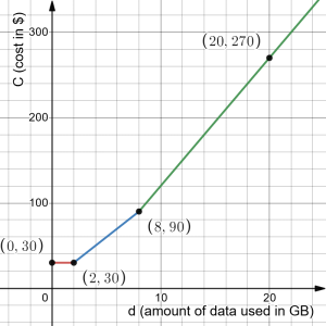
A phone data plan has a basic charge of $30 a month. The plan includes first 2GB free and charges $10 for each additional GB, up to 8 GB total usage, after which it charges $15 for each additional GB. If [latex]d[/latex] is the amount of data used (in GB) and [latex]C[/latex] is the total monthly cost:
a. Express [latex]C(d)[/latex] as a (piece-wise) formula.
b. Identify the domain and range of [latex]C(d)[/latex].
c. Graph [latex]C[/latex] as a function of [latex]d[/latex] for [latex]0\le d\le 10[/latex].
d. Calculate the cost if 9GB were used.
Answer:
a. Task: [latex]C(d)=?[/latex]
Conditions:
only basic charge for first 2GB [latex]\Rightarrow C(d)=\underbrace{30}_{\text{basic charge}}, 0\le d\le 2[/latex]
after 2GB and up to 8 GB, charge of $10/GB for additional GB
[latex]\Rightarrow C(d)=\underbrace{30}_{\text{cost of first 2GB}}+\underbrace{10(d-2)}_{\text{cost above 2GB}}=10d+10, 2< d\le 8[/latex]
after 8GB, charge of $15/GB for additional GB
[latex]\Rightarrow C(d)=\underbrace{30+10(8-2)}_{\text{cost of first 8GB}}+\underbrace{15(d-8)}_{\text{cost above 8GB}}=15d-30, 2< d\le 8[/latex]
In piece-wise form:
[latex]C(d)=\begin{cases} 30 & 0\le d\le 2 \\ 10d+10& 2< d\le 8 \\ 15d-30 & 8< d \end{cases}[/latex] b. domain? [latex]\to[/latex] all possible input values, where the input is amount of data used [latex]d[/latex]
Mathematically, [latex]C(d)[/latex] can be calculated for any value of [latex]d[/latex] so [latex]d[/latex] can be any real number.
Contextually, [latex]d=\text{amount of data used}\rightarrow[/latex] can't be negative, and has no upper limit [latex]\Rightarrow d\ge 0[/latex]
Hence, the domain is [latex][0,\infty)[/latex]
range? [latex]\to[/latex] all possible output values, where the output is cost [latex]C(d)[/latex]
Since the cost is at least 30 and increasing as [latex]d[/latex] increases with no upper limit [latex]\Rightarrow C(d)\ge 30[/latex]
Therefore, the range is [latex][30,\infty)[/latex].
c. Each section is a linear function so we can graph each section by finding two points that belong to the respective lines:
[latex]\begin{align*} 0\le d\le 2&:C(0)=30; C(2)=30\\ 2< d\le 8&: C(2)=10\cdot 2+10=30; C(8)=10\cdot 8+10=90\\ d>8&:C(8)=15\cdot 8-30=90; C(20)=15\cdot 20-30=270 \end{align*}[/latex]
(Note that for the last section our choice for 20 as input was arbitrary; we could have picked any number greater than 8.)
So the graph looks as follows:
d. [latex]C(9)=?[/latex]
Since [latex]9>8[/latex], [latex]C(d)=15d-30[/latex] applies and so [latex]C(9)=15\cdot 9-30=105[/latex]. Hence the cost if 9GB are used is $105.
Sometimes we can expand the rule we are given between some restricted sets of data to create new functions, which might provide us with a greater insight into the relationship we are studying, through so called data modeling. In this case, not only would the rule of the function be potentially adjusted, but also the function's domain and range.
For example, the table below shows a relationship between the circumference and the height of a tree as it grows.
| Circumference, [latex]c[/latex] (feet) | 1.7 | 2.5 | 5.5 | 8.2 | 13.7 |
| Height, [latex]h[/latex] (feet) | 24.5 | 31 | 45.2 | 54.6 | 92.1 |
While there is a strong relationship between the two, it would certainly be ridiculous to talk about a tree with a circumference of -3 feet, or a height of 3000 feet. When we identify limitations on the inputs and outputs of a function, we are determining the domain and range of the function. In this particular case, the domain is, strictly speaking, the set of circumference values that give us a height value. In other words:
domain of [latex]h(c)[/latex] is [latex]\{1.7, 2.5, 5.5, 8.2, 13.7\}[/latex]
range of [latex]h(c)[/latex] is [latex]\{24.5, 31, 45.2, 54.6, 92.1\}[/latex]
It is natural to assume that some other values for the circumference of the tree would give us an associated height. Yet we don't have that information so we cannot include it in this particular function. However, there are mathematical methods we could use to interpolate (fill in the missing data) and extrapolate (predict beyond given boundaries of the data) to create a function that models the given data and allows us to make inferences about this relationship. In this model, the domain and the potentially range of this new function would be bigger than the domain and the range of the original [latex]h(c)[/latex] function. See the example below for a demonstration.
Example 12
Using the tree table above, determine a function that would provide a reasonable model for the given data, and describe its domain and range.
Answer:
Model: Using the data we were given on the tree circumference and height relationship
| Circumference, [latex]c[/latex] (feet) | 1.7 | 2.5 | 5.5 | 8.2 | 13.7 |
| Height, [latex]h[/latex] (feet) | 24.5 | 31 | 45.2 | 54.6 | 92.1 |
we can use the mathematical method called linear regression. For example, using the graphing tool Desmos, we can produce the following model for [latex]h(c)[/latex]:
[latex]h(c)=14.7005c^{0.683083}[/latex]
You can view this model here: https://www.desmos.com/calculator/wizo7fwqcy
Domain: To determine the domain of this model we would have to consider all possible input values, both mathematically and contextually.
Mathematically, in the formula for the model, the values of [latex]c[/latex] cannot be negative (try this by calculating [latex]h(c)[/latex] for some negative value of [latex]c[/latex]). Therefore, the input values must be non-negative, i.e., [latex]c\ge 0[/latex].
Contextually, however, we have to think about the meaning of the input and the output values produced by the input.
Input values within the context: Since the input values represent the circumference of the tree, it makes sense to only allow non-negative values for [latex]c[/latex], and so [latex]c \ge 0[/latex]. Additionally, it is reasonable to assume that the circumference of a tree cannot be arbitrarily large, so we could make an informed guess at a maximum reasonable value. Looking up that information, we find that the maximum tree circumference measured is about 119 feet, so let's approximate it to 120 feet. In other words, within the context of the independent variable representing the inputs, the reasonable input values are [latex]0\le c\le 120[/latex].
Output values produced within the context: We would also have to make sure that the input values produce contextually reasonable outputs. In particular, the height when the circumference is 0 should also be zero, which is the case in this model, so the zero circumference is in the domain, i.e, [latex]c=0[/latex] is contextually a possible input. Moreover, these values should produce non-negative heights and they should not be ridiculously large. Since the formula produces positive values if the input value is positive, all positive values of [latex]c[/latex] will produce a positive value for [latex]h[/latex], or the height. To consider the restriction on maximum height, by looking at the graph of this model we can see that the height continually increases as the circumference increases (which is what we would expect in nature, so that's good). Therefore, by using our formula for the model, we can see that the circumference value of [latex]c=120[/latex] will give us the height value of [latex]h(120)=14.7005\cdot(120)^{0.683083}\approx 387[/latex]. Looking up information on the tallest tree ever recorded, we can see that record is about 380 feet, and so our model seems contextually reasonable for the input values of [latex]c[/latex] being at least 0 and up to 120 feet.
Considering now the restrictions on the domain both mathematically and contextually, we can conclude that a reasonable domain for the function modeling this data is all real numbers from 0 to 120, inclusively. Mathematically we would write this as [latex][0,120][/latex] or [latex]\{c\in\mathbb{R}\vert 0\le c\le 120\}[/latex].
Range: The range is all possible output values and so, since the inputs can be any values from 0 to 120 and the function is increasing without any breaks between those two input values, the range will be all values between [latex]h(0)[/latex] and [latex]h(120)[/latex], i.e., all values between 0 and approximately 387.
Summary Concept Check
Test your understanding of the concepts discussed in this section: Interactive demo on MathMatize
Section Exercises
Work on the following exercises. Discuss your solutions with your peers and/or course instructor.
