6.4 – Operational Amplifiers – Charts and Math

Operational Amplifiers – Gain Bandwidth Product (GBP)

The open loop frequency response of a general-purpose op amp is shown in Figure 6.4.2 . Although the exact frequency and gain values will differ from model to model, all devices will exhibit this same general shape and 20 dB per decade roll-off slope. This is because the lag break frequency ([latex]f_d[/latex]) is determined by a single capacitor called the compensation capacitor. This capacitor is usually in the Miller position (i.e., straddling input and output) of an intermediate stage. Although this capacitor is rather small, the Miller effect drastically increases its apparent value. The resulting critical frequency is very low, often in the range of 10 to 100 Hz. The other circuit lag networks caused by stray or load capacitances are much higher, usually over 1 MHz. As a result, a constant 20 dB per decade roll-off is maintained from [latex]f_c[/latex] up to very high frequencies. The remaining lag networks will not affect the open-loop response until the gain has already dropped below zero dB.

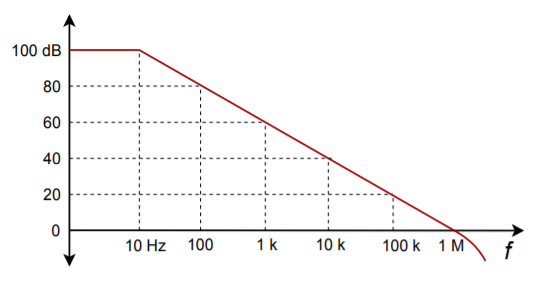
Figure 6.4.1 – Open loop frequency response

This type of frequency response curve has two benefits: (1) The most important benefit is that it allows you to set almost any gain you desire with stability. Only a single network is active, thus satisfactory gain and phase margins will be maintained. Therefore, your negative feedback never turns into positive feedback 2) The product of any break frequency and its corresponding gain is a constant. In other words, the gain decreases at the same rate at which the frequency increases. In Figure 5.3.1 , the product is 1 MHz. As you might have guessed, this parameter is the gain-bandwidth product of the op amp (GBW). GBW is also referred to as [latex]\text{funity}[/latex] (the frequency at which the open loop gain equals one).

From this frequency response curve shown above, we can see that the product of the gain against frequency is constant at any point along the curve. Also that the unity gain (0dB) frequency also determines the gain of the amplifier at any point along the curve. This constant is generally known as the Gain Bandwidth Product or GBP. Therefore:

[latex]{GPB} = \text{Gain} \cdot \text{Bandwidth} = A \cdot {BW}[/latex]

For example, from the graph above the gain of the amplifier at 100kHz is given as 20dB or 10, then the gain bandwidth product is calculated as:

[latex]{GPB} = A \cdot {BW} = 10 \times 100000\, \text{Hz} = 1000000\, \text{Hz}[/latex]

Similarly, the operational amplifiers gain at 1kHz = 60dB or 1000, therefore the GBP is given as:

[latex]{GPB} = A \cdot {BW} = 1000 \times 1000\, \text{Hz} = 1000000\, \text{Hz}[/latex] The same!

The Voltage Gain (AV) of the operational amplifier can be found using the following formula:

[latex]A = \frac{V_\text{out}}{V_\text{in}}[/latex]

and in Decibels or (dB) is given as:

[latex]20 \log\left(\frac{V_{\text{out}}}{V_{\text{in}}}\right)[/latex]

Operational Amplifiers Bandwidth

The operational amplifiers bandwidth is the frequency range over which the voltage gain of the amplifier is above 70.7% or 3dB (where 0dB is the maximum) of its maximum output value as shown below.

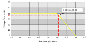
Figure 6.4.2 – Graph plotting frequency against voltage gain for operational amplifiers

Example 1

Using the formula [latex]20 \log A[/latex], we can calculate the bandwidth of the amplifier as:

Then the bandwidth of the amplifier at a gain of 40dB is given as 14kHz as previously predicted from the graph.

Example 2

If the gain of the operational amplifier was reduced by half, lets say to 20dB, in the above frequency response curve, the -3dB point would now be at 17dB. This would then give the operational amplifier an overall gain of 7.08, therefore A = 7.08.

If we use the same formula as above, this new gain would give us a bandwidth of approximately 141.2kHz, ten times more than the frequency given at the 40dB point. It can therefore be seen that by reducing the overall “open loop gain” of an operational amplifier its bandwidth is increased and visa versa.

In other words, an operational amplifiers bandwidth is inversely proportional to its gain, ( A 1/∝ BW ). Also, this -3dB corner frequency point is generally known as the “half power point”, as the output power of the amplifier is at half its maximum value as shown: