Chapter 4.3: The Derivative as a Function
Learning Objectives
- Define the derivative function of a given function.
- Graph a derivative function from the graph of a given function.
- State the connection between derivatives and continuity.
- Describe three conditions for when a function does not have a derivative.
- Explain the meaning of a higher-order derivative.
As we have seen, the derivative of a function at a given point gives us the rate of change or slope of the tangent line to the function at that point. If we differentiate a position function at a given time, we obtain the velocity at that time. It seems reasonable to conclude that knowing the derivative of the function at every point would produce valuable information about the behavior of the function. However, the process of finding the derivative at even a handful of values using the techniques of the preceding section would quickly become quite tedious. In this section we define the derivative function and learn a process for finding it.
Derivative Functions
The derivative function gives the derivative of a function at each point in the domain of the original function for which the derivative is defined. We can formally define a derivative function as follows.
Definition
Let  be a function. The derivative function, denoted by
  , is the function whose domain consists of those values of
  such that the following limit exists:
 .
.A function  is said to be differentiable at
  if
if
 exists. More generally, a function is said to be differentiable on
  if it is differentiable at every point in an open set , and a differentiable function is one in which
  exists on its domain.
In the next few examples we use (Figure) to find the derivative of a function.
Finding the Derivative of a Square-Root Function
Find the derivative of  .
.

Finding the Derivative of a Quadratic Function
Find the derivative of the function  .
.
Solution
Follow the same procedure here, but without having to multiply by the conjugate.

Find the derivative of  .
.
Solution

We use a variety of different notations to express the derivative of a function. In (Figure) we showed that if , then  . If we had expressed this function in the form
  , we could have expressed the derivative as
  or
or  . We could have conveyed the same information by writing
  . Thus, for the function
  , each of the following notations represents the derivative of :
 .
.In place of we may also use  Use of the
  notation (called Leibniz notation) is quite common in engineering and physics. To understand this notation better, recall that the derivative of a function at a point is the limit of the slopes of secant lines as the secant lines approach the tangent line. The slopes of these secant lines are often expressed in the form
  where
where  is the difference in the
  values corresponding to the difference in the values, which are expressed as
  ((Figure)). Thus the derivative, which can be thought of as the instantaneous rate of change of with respect to , is expressed as
 .
.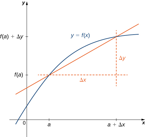 .
.Graphing a Derivative
We have already discussed how to graph a function, so given the equation of a function or the equation of a derivative function, we could graph it. Given both, we would expect to see a correspondence between the graphs of these two functions, since gives the rate of change of a function (or slope of the tangent line to ).
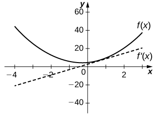
In (Figure) we found that for  . If we graph these functions on the same axes, as in (Figure), we can use the graphs to understand the relationship between these two functions. First, we notice that is increasing over its entire domain, which means that the slopes of its tangent lines at all points are positive. Consequently, we expect
  for all values of in its domain. Furthermore, as increases, the slopes of the tangent lines to are decreasing and we expect to see a corresponding decrease in . We also observe that
  is undefined and that
  , corresponding to a vertical tangent to at 0.
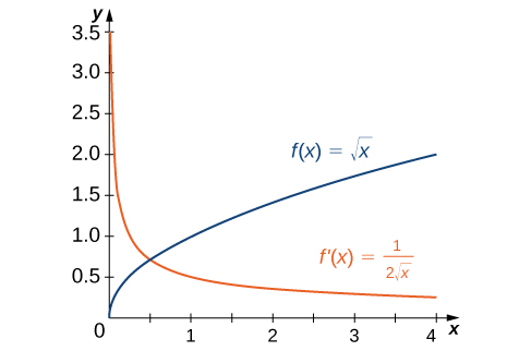 is positive everywhere because the function is increasing.
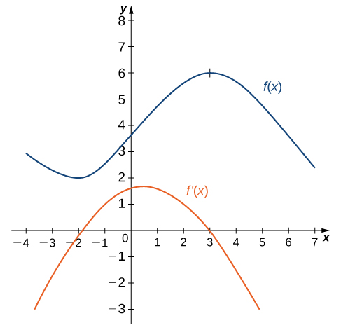
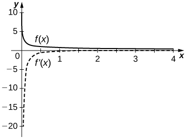
In (Figure) we found that for  . The graphs of these functions are shown in (Figure). Observe that is decreasing for
  . For these same values of
  . For values of
  is increasing and . Also, has a horizontal tangent at
  and
and  .
.
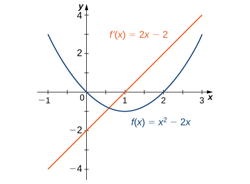
 where the function is decreasing and where is increasing. The derivative is zero where the function has a horizontal tangent.
Sketching a Derivative Using a Function
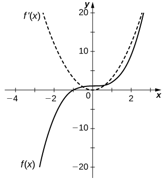
Use the following graph of to sketch a graph of .
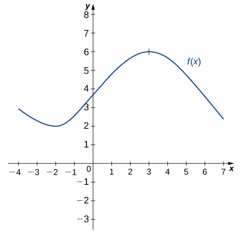
Solution
The solution is shown in the following graph. Observe that is increasing and on  . Also, is decreasing and on
  and on
  . Also note that has horizontal tangents at -2 and 3, and
  and
and  .
.
Sketch the graph of  . On what interval is the graph of above the -axis?
Solution

Hint
The graph of is positive where is increasing.
Derivatives and Continuity
Now that we can graph a derivative, let’s examine the behavior of the graphs. First, we consider the relationship between differentiability and continuity. We will see that if a function is differentiable at a point, it must be continuous there; however, a function that is continuous at a point need not be differentiable at that point. In fact, a function may be continuous at a point and fail to be differentiable at the point for one of several reasons.
Differentiability Implies Continuity
Let be a function and be in its domain. If is differentiable at , then is continuous at .
Proof
If is differentiable at , then exists and
 .
.We want to show that is continuous at by showing that  . Thus,

Therefore, since  is defined and , we conclude that is continuous at .
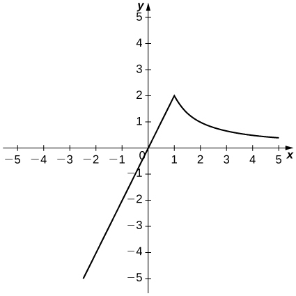
We have just proven that differentiability implies continuity, but now we consider whether continuity implies differentiability. To determine an answer to this question, we examine the function  . This function is continuous everywhere; however,
  is undefined. This observation leads us to believe that continuity does not imply differentiability. Let’s explore further. For ,
 .
.This limit does not exist because
 .
.See (Figure).
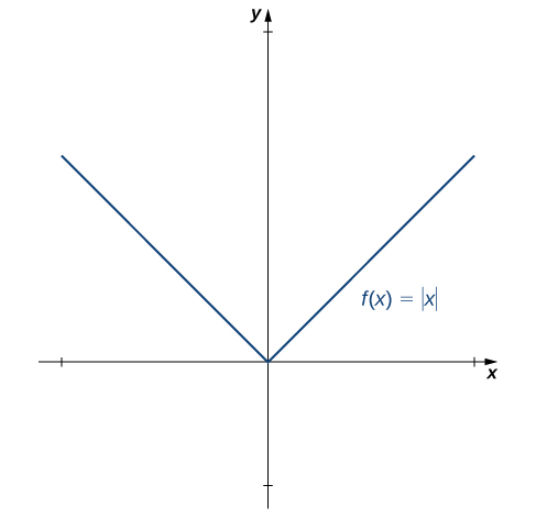 is continuous at 0 but is not differentiable at 0.
Let’s consider some additional situations in which a continuous function fails to be differentiable. Consider the function ![f(x)=\sqrt[3]{x}](https://ecampusontario.pressbooks.pub/app/uploads/quicklatex/quicklatex.com-c3c5e7be9bc257eb2866277bae5be644_l3.png "Rendered by QuickLaTeX.com") :
:
![f^{\prime}(0)=\underset{x\to 0}{\lim}\frac{\sqrt[3]{x}-0}{x-0}=\underset{x\to 0}{\lim}\frac{1}{\sqrt[3]{x^2}}=+\infty](https://ecampusontario.pressbooks.pub/app/uploads/quicklatex/quicklatex.com-a4d285748e36cb68cb88297a08c9bfb8_l3.png "Rendered by QuickLaTeX.com") .
.Thus does not exist. A quick look at the graph of clarifies the situation. The function has a vertical tangent line at 0 ((Figure)).
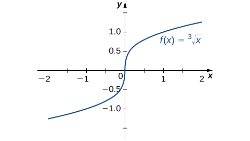 has a vertical tangent at
  . It is continuous at 0 but is not differentiable at 0.
The function  also has a derivative that exhibits interesting behavior at 0. We see that
 .
.This limit does not exist, essentially because the slopes of the secant lines continuously change direction as they approach zero ((Figure)).
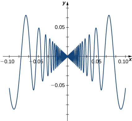 is not differentiable at 0.
In summary:
- We observe that if a function is not continuous, it cannot be differentiable, since every differentiable function must be continuous. However, if a function is continuous, it may still fail to be differentiable.
- We saw that failed to be differentiable at 0 because the limit of the slopes of the tangent lines on the left and right were not the same. Visually, this resulted in a sharp corner on the graph of the function at 0. From this we conclude that in order to be differentiable at a point, a function must be “smooth” at that point.
- As we saw in the example of , a function fails to be differentiable at a point where there is a vertical tangent line.
- As we saw with a function may fail to be differentiable at a point in more complicated ways as well.
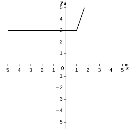
A Piecewise Function that is Continuous and Differentiable
A toy company wants to design a track for a toy car that starts out along a parabolic curve and then converts to a straight line ((Figure)). The function that describes the track is to have the form  , where and are in inches. For the car to move smoothly along the track, the function must be both continuous and differentiable at -10. Find values of
  and
and  that make both continuous and differentiable.
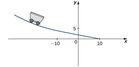
Solution
For the function to be continuous at  . Thus, since

and  , we must have
  . Equivalently, we have
  .
.
For the function to be differentiable at -10,

must exist. Since is defined using different rules on the right and the left, we must evaluate this limit from the right and the left and then set them equal to each other:

We also have

This gives us  . Thus
  and
and  .
.
Find values of and that make  both continuous and differentiable at 3.
Solution
 and
and 
Hint
Use (Figure) as a guide.
Higher-Order Derivatives
The derivative of a function is itself a function, so we can find the derivative of a derivative. For example, the derivative of a position function is the rate of change of position, or velocity. The derivative of velocity is the rate of change of velocity, which is acceleration. The new function obtained by differentiating the derivative is called the second derivative. Furthermore, we can continue to take derivatives to obtain the third derivative, fourth derivative, and so on. Collectively, these are referred to as higher-order derivatives. The notation for the higher-order derivatives of can be expressed in any of the following forms:


 .
.It is interesting to note that the notation for  may be viewed as an attempt to express
  more compactly. Analogously,
  .
.
Finding a Second Derivative
For  , find
  .
.
Solution
First find .

Next, find by taking the derivative of  .
.


Finding Acceleration
The position of a particle along a coordinate axis at time  (in seconds) is given by
  (in meters). Find the function that describes its acceleration at time .
Solution
Since  and
and  , we begin by finding the derivative of
  :
:

Next,

Thus,  .
.
 , find
  .
.
Key Concepts
- The derivative of a function is the function whose value at is .
- The graph of a derivative of a function is related to the graph of . Where has a tangent line with positive slope, . Where has a tangent line with negative slope, . Where has a horizontal tangent line,
 .
. - If a function is differentiable at a point, then it is continuous at that point. A function is not differentiable at a point if it is not continuous at the point, if it has a vertical tangent line at the point, or if the graph has a sharp corner or cusp.
- Higher-order derivatives are derivatives of derivatives, from the second derivative to the
 derivative.
Key Equations
- The derivative function
For the following exercises, use the definition of a derivative to find .
1. 
2. 
Solution
-3
3. 
4. 
Solution

5. 
6. 
Solution

7. 
8. 
Solution

9. 
10. 
Solution

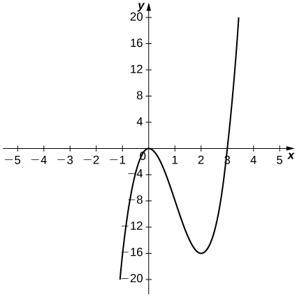
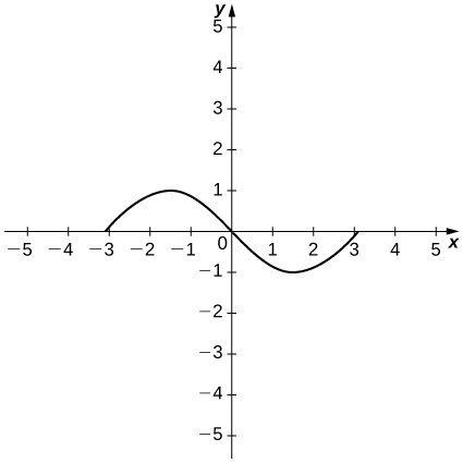
For the following exercises, use the graph of to sketch the graph of its derivative .
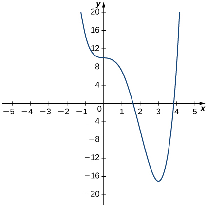
Solution
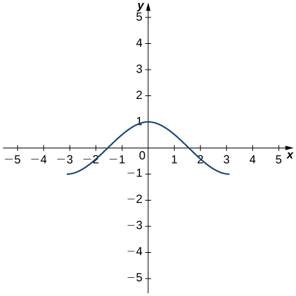
Solution
For the following exercises, the given limit represents the derivative of a function at  . Find and .
15. 
16. ![\underset{h\to 0}{\lim}\frac{[3(2+h)^2+2]-14}{h}](https://ecampusontario.pressbooks.pub/app/uploads/quicklatex/quicklatex.com-79c2acf739434ece433b8f58488be22e_l3.png "Rendered by QuickLaTeX.com")
Solution

17. 
18. 
Solution

19. ![\underset{h\to 0}{\lim}\frac{[2(3+h)^2-(3+h)]-15}{h}](https://ecampusontario.pressbooks.pub/app/uploads/quicklatex/quicklatex.com-c04662eed627ce29150a859b2d400036_l3.png "Rendered by QuickLaTeX.com")
20. 
Solution

For the following functions,
- sketch the graph and
- use the definition of a derivative to show that the function is not differentiable at .
21. 
22. 
Solution
a.
b. 
23. 
24. 
Solution
a.
b.  .
.
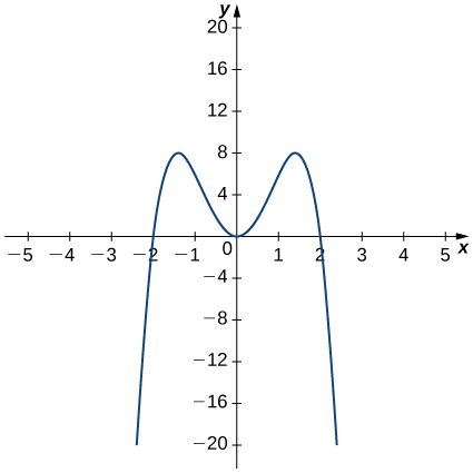
For the following graphs,
- determine for which values of the
 exists but is not continuous at , and
 - determine for which values of the function is continuous but not differentiable at .
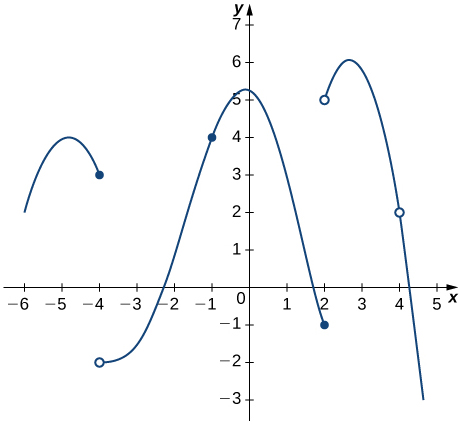
Solution
a. , b. 
27. Use the graph to evaluate a.  , b. , c.
  , d.
, d.  , and e.
  , if they exist.
For the following functions, use  to find .
28.
Solution
0
29.
30.
Solution

For the following exercises, use a calculator to graph . Determine the function , then use a calculator to graph .
31. [T] 
32. [T] 
Solution

33. [T] 
34. [T] 
Solution

35. [T] 
36. [T] 
Solution

For the following exercises, describe what the two expressions represent in terms of each of the given situations. Be sure to include units.

37.  denotes the population of a city at time in years.
38.  denotes the total amount of money (in thousands of dollars) spent on concessions by customers at an amusement park.
Solution
a. Average rate at which customers spent on concessions in thousands per customer.
b. Rate (in thousands per customer) at which customers spent money on concessions in thousands per customer.
39.  denotes the total cost (in thousands of dollars) of manufacturing clock radios.
40.  denotes the grade (in percentage points) received on a test, given hours of studying.
Solution
a. Average grade received on the test with an average study time between two amounts.
b. Rate (in percentage points per hour) at which the grade on the test increased or decreased for a given average study time of hours.
41.  denotes the cost (in dollars) of a sociology textbook at university bookstores in the United States in years since 1990.
42.  denotes atmospheric pressure at an altitude of feet.
Solution
a. Average change of atmospheric pressure between two different altitudes.
b. Rate (torr per foot) at which atmospheric pressure is increasing or decreasing at feet.
43. Sketch the graph of a function with all of the following properties:
- for

-

- for

-
 and
and 
-
 and
and 
- does not exist.
44. Suppose temperature  in degrees Fahrenheit at a height in feet above the ground is given by
  .
.
- Give a physical interpretation, with units, of
 .
. - If we know that
 explain the physical meaning.
Solution
a. The rate (in degrees per foot) at which temperature is increasing or decreasing for a given height .
b. The rate of change of temperature as altitude changes at 1000 feet is -0.1 degrees per foot.
45. Suppose the total profit of a company is  thousand dollars when units of an item are sold.
- What does
 for
for  measure, and what are the units?
 - What does
 measure, and what are the units?
 - Suppose that
 . What is the approximate change in profit if the number of items sold increases from 30 to 31?
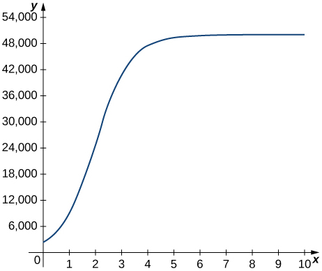
46. The graph in the following figure models the number of people  who have come down with the flu weeks after its initial outbreak in a town with a population of 50,000 citizens.
- Describe what
 represents and how it behaves as increases.
 - What does the derivative tell us about how this town is affected by the flu outbreak?
Solution
a. The rate at which the number of people who have come down with the flu is changing weeks after the initial outbreak.
b. The rate is increasing sharply up to the third week, at which point it slows down and then becomes constant.
For the following exercises, use the following table, which shows the height  of the Saturn V rocket for the Apollo 11 mission seconds after launch.
| Time (seconds) | Height (meters) |
|---|---|
| 0 | 0 |
| 1 | 2 |
| 2 | 4 |
| 3 | 13 |
| 4 | 25 |
| 5 | 32 |
47. What is the physical meaning of  ? What are the units?
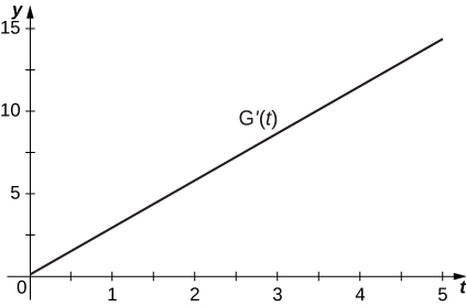
48. [T] Construct a table of values for and graph both  and on the same graph. (Hint: for interior points, estimate both the left limit and right limit and average them.)
Solution
| Time (seconds) | (m/s) |
|---|---|
| 0 | 2 |
| 1 | 2 |
| 2 | 5.5 |
| 3 | 10.5 |
| 4 | 9.5 |
| 5 | 7 |
49. [T] The best linear fit to the data is given by  , where
  is the height of the rocket (in meters) and is the time elapsed since takeoff. From this equation, determine
  . Graph
  with the given data and, on a separate coordinate plane, graph .
50. [T] The best quadratic fit to the data is given by  , where
  is the height of the rocket (in meters) and is the time elapsed since takeoff. From this equation, determine
  . Graph
  with the given data and, on a separate coordinate plane, graph .
Solution

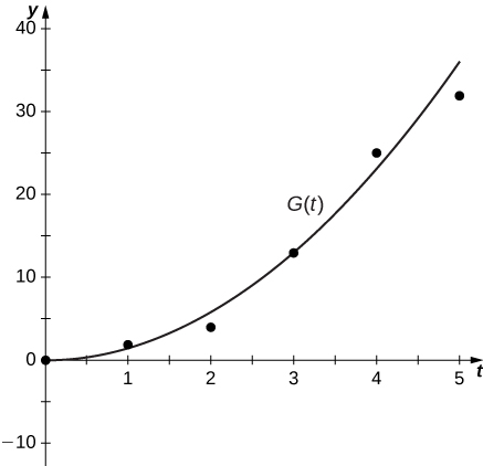
51. [T] The best cubic fit to the data is given by  , where
  is the height of the rocket (in m) and is the time elapsed since take off. From this equation, determine
  . Graph
  with the given data and, on a separate coordinate plane, graph . Does the linear, quadratic, or cubic function fit the data best?
52. Using the best linear, quadratic, and cubic fits to the data, determine what  , and
, and  are. What are the physical meanings of , and , and what are their units?
Solution
 , and
, and  represent the acceleration of the rocket, with units of meters per second squared (
  ).
).
Glossary
- derivative function
- gives the derivative of a function at each point in the domain of the original function for which the derivative is defined
- differentiable at
- a function for which exists is differentiable at
- differentiable on
- a function for which exists for each in the open set is differentiable on
- differentiable function
- a function for which exists is a differentiable function
- higher-order derivative
- a derivative of a derivative, from the second derivative to the
 th derivative, is called a higher-order derivative

Hint
Use (Figure) and follow the example.