Chapter 2.6: Exponential and Logarithmic Functions
Learning Objectives
- Identify the form of an exponential function.
- Explain the difference between the graphs of
 and
and  .
. - Recognize the significance of the number
 .
. - Identify the form of a logarithmic function.
- Explain the relationship between exponential and logarithmic functions.
- Describe how to calculate a logarithm to a different base.
- Identify the hyperbolic functions, their graphs, and basic identities.
In this section we examine exponential and logarithmic functions. We use the properties of these functions to solve equations involving exponential or logarithmic terms, and we study the meaning and importance of the number . We also define hyperbolic and inverse hyperbolic functions, which involve combinations of exponential and logarithmic functions. (Note that we present alternative definitions of exponential and logarithmic functions in the chapter Applications of Integrations, and prove that the functions have the same properties with either definition.)
Exponential Functions
Exponential functions arise in many applications. One common example is population growth.
For example, if a population starts with  individuals and then grows at an annual rate of
  , its population after 1 year is
 .
.Its population after 2 years is
 .
.In general, its population after  years is
 ,
,which is an exponential function. More generally, any function of the form  , where
  , is an exponential function with base
  and exponent
  . Exponential functions have constant bases and variable exponents. Note that a function of the form
  for some constant is not an exponential function but a power function.
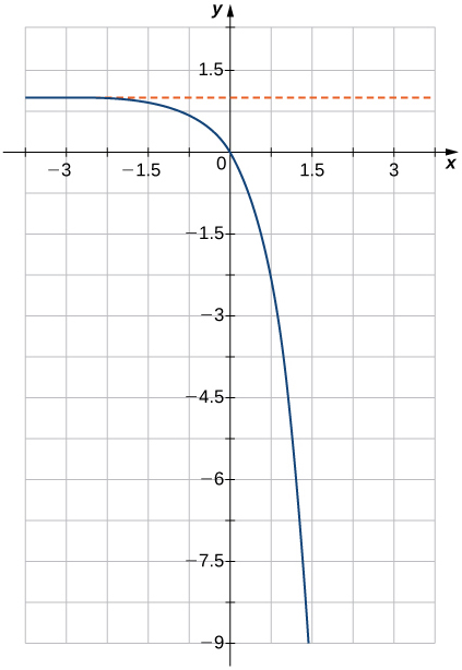
To see the difference between an exponential function and a power function, we compare the functions  and
and  . In (Figure), we see that both
  and
and  approach infinity as
  . Eventually, however, becomes larger than and grows more rapidly as . In the opposite direction, as
  , whereas
  . The line
  is a horizontal asymptote for .
 |
-3 | -2 | -1 | 0 | 1 | 2 | 3 | 4 | 5 | 6 |
 |
9 | 4 | 1 | 0 | 1 | 4 | 9 | 16 | 25 | 36 |
 |
 |
 |
 |
1 | 2 | 4 | 8 | 16 | 32 | 64 |
In (Figure), we graph both and to show how the graphs differ.
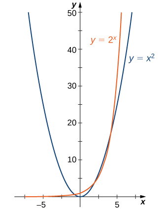 and approach infinity as , but grows more rapidly than . As , whereas .
Evaluating Exponential Functions
Recall the properties of exponents: If is a positive integer, then we define  (with factors of ). If is a negative integer, then
  for some positive integer
  , and we define
  . Also,
  is defined to be 1. If is a rational number, then
  , where
  and
and  are integers and
 ![b^x=b^{p/q}=\sqrt[q]{b^p}](https://ecampusontario.pressbooks.pub/app/uploads/quicklatex/quicklatex.com-14bb58a36abbf1a68b48d6dd2157d326_l3.png "Rendered by QuickLaTeX.com") . For example,
. For example,  . However, how is defined if is an irrational number? For example, what do we mean by
  ? This is too complex a question for us to answer fully right now; however, we can make an approximation. In (Figure), we list some rational numbers approaching
  , and the values of for each rational number are presented as well. We claim that if we choose rational numbers getting closer and closer to , the values of get closer and closer to some number
  . We define that number to be .
| |
1.4 | 1.41 | 1.414 | 1.4142 | 1.41421 | 1.414213 |
| |
2.639 | 2.65737 | 2.66475 | 2.665119 | 2.665138 | 2.665143 |
Bacterial Growth
Suppose a particular population of bacteria is known to double in size every 4 hours. If a culture starts with 1000 bacteria, the number of bacteria after 4 hours is  . The number of bacteria after 8 hours is
  . In general, the number of bacteria after
  hours is
  . Letting
  , we see that the number of bacteria after hours is
  . Find the number of bacteria after 6 hours, 10 hours, and 24 hours.
Solution
The number of bacteria after 6 hours is given by  bacteria. The number of bacteria after 10 hours is given by
  bacteria. The number of bacteria after 24 hours is given by
  bacteria.
Given the exponential function  , evaluate
  and
and  .
.
Solution
 .
.
Go to World Population Balance for another example of exponential population growth.
Graphing Exponential Functions
For any base  , the exponential function is defined for all real numbers and
  . Therefore, the domain of is
  and the range is
  . To graph , we note that for
  is increasing on and
  as , whereas
  as
as  . On the other hand, if
  is decreasing on and as
  whereas as
  ((Figure)).
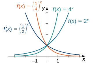
 , then is increasing on . If
  , then is decreasing on .
Visit this site for more exploration of the graphs of exponential functions.
Note that exponential functions satisfy the general laws of exponents. To remind you of these laws, we state them as rules.
Rule: Laws of Exponents
For any constants  , and for all and ,


Using the Laws of Exponents
Use the laws of exponents to simplify each of the following expressions.


Solution
- We can simplify as follows:
 .
. - We can simplify as follows:
 .
.
Use the laws of exponents to simplify  .
.
Solution

The Number
A special type of exponential function appears frequently in real-world applications. To describe it, consider the following example of exponential growth, which arises from compounding interest in a savings account. Suppose a person invests  dollars in a savings account with an annual interest rate
  , compounded annually. The amount of money after 1 year is
 .
.The amount of money after 2 years is
 .
.More generally, the amount after years is
 .
.If the money is compounded 2 times per year, the amount of money after half a year is
 .
.The amount of money after 1 year is
 .
.After years, the amount of money in the account is
 .
.More generally, if the money is compounded  times per year, the amount of money in the account after years is given by the function
 .
.What happens as  ? To answer this question, we let
  and write
 ,
,and examine the behavior of  as
as  , using a table of values ((Figure)).
 |
10 | 100 | 1000 | 10,000 | 100,000 | 1,000,000 |
 |
2.5937 | 2.7048 | 2.71692 | 2.71815 | 2.718268 | 2.718280 |
 as
as 
Looking at this table, it appears that is approaching a number between 2.7 and 2.8 as  . In fact, does approach some number as . We call this number . To six decimal places of accuracy,
 .
.The letter was first used to represent this number by the Swiss mathematician Leonhard Euler during the 1720s. Although Euler did not discover the number, he showed many important connections between and logarithmic functions. We still use the notation today to honor Euler’s work because it appears in many areas of mathematics and because we can use it in many practical applications.
Returning to our savings account example, we can conclude that if a person puts dollars in an account at an annual interest rate , compounded continuously, then  . This function may be familiar. Since functions involving base arise often in applications, we call the function
  the natural exponential function. Not only is this function interesting because of the definition of the number , but also, as discussed next, its graph has an important property.
Since  , we know
  is increasing on . In (Figure), we show a graph of along with a tangent line to the graph of at
  . We give a precise definition of tangent line in the next chapter; but, informally, we say a tangent line to a graph of
  at
at  is a line that passes through the point
  and has the same “slope” as at that point. The function is the only exponential function with tangent line at that has a slope of 1. As we see later in the text, having this property makes the natural exponential function the simplest exponential function to use in many instances.
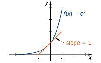 has a tangent line with slope 1 at .
Compounding Interest
Suppose  is invested in an account at an annual interest rate of
  , compounded continuously.
- Let denote the number of years after the initial investment and
 denote the amount of money in the account at time . Find a formula for .
 - Find the amount of money in the account after 10 years and after 20 years.
Solution
- If dollars are invested in an account at an annual interest rate , compounded continuously, then . Here
 and
and  . Therefore,
  .
. - After 10 years, the amount of money in the account is
 .
.After 20 years, the amount of money in the account is
 .
.
If  is invested in an account at an annual interest rate of
  , compounded continuously, find a formula for the amount of money in the account after years. Find the amount of money after 30 years.
Show Answer
 . After 30 years, there will be approximately
  .
.
Hint
.
Logarithmic Functions
Using our understanding of exponential functions, we can discuss their inverses, which are the logarithmic functions. These come in handy when we need to consider any phenomenon that varies over a wide range of values, such as pH in chemistry or decibels in sound levels.
The exponential function is one-to-one, with domain and range  . Therefore, it has an inverse function, called the logarithmic function with base . For any , the logarithmic function with base , denoted
  , has domain and range
  , and satisfies
 if and only if
  .
.For example,

Furthermore, since  and
and  are inverse functions,
 .
.The most commonly used logarithmic function is the function  . Since this function uses natural as its base, it is called the natural logarithm. Here we use the notation
  or
or  to mean . For example,
 .
.Since the functions and  are inverses of each other,
 ,
,and their graphs are symmetric about the line  ((Figure)).
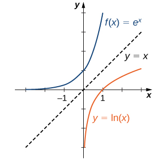
 and
and  are inverses of each other, so their graphs are symmetric about the line .
At this site you can see an example of a base-10 logarithmic scale.
In general, for any base , the function  is symmetric about the line with the function . Using this fact and the graphs of the exponential functions, we graph functions
  for several values of ((Figure)).
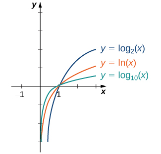 are depicted for
  .
.Before solving some equations involving exponential and logarithmic functions, let’s review the basic properties of logarithms.
Rule: Properties of Logarithms
If  , and is any real number, then

Solving Equations Involving Exponential Functions
Solve each of the following equations for .


Solution
- Applying the natural logarithm function to both sides of the equation, we have
 .
.Using the power property of logarithms,
 .
.Therefore,
 .
. - Multiplying both sides of the equation by , we arrive at the equation
 .
.Rewriting this equation as
 ,
,we can then rewrite it as a quadratic equation in
: .
.Now we can solve the quadratic equation. Factoring this equation, we obtain
 .
.Therefore, the solutions satisfy
 and
and  . Taking the natural logarithm of both sides gives us the solutions
  .
.
Solve  .
.
Solution

Hint
First solve the equation for  .
.
Solving Equations Involving Logarithmic Functions
Solve each of the following equations for .


Solution
- By the definition of the natural logarithm function,
 .
.Therefore, the solution is
 .
. - Using the product and power properties of logarithmic functions, rewrite the left-hand side of the equation as
 .
.Therefore, the equation can be rewritten as
 .
.The solution is
![x=10^{4/3}=10\sqrt[3]{10}](https://ecampusontario.pressbooks.pub/app/uploads/quicklatex/quicklatex.com-88984457a8787d6d370b8c0fd05f2568_l3.png "Rendered by QuickLaTeX.com") .
. - Using the power property of logarithmic functions, we can rewrite the equation as
 .
.
Using the quotient property, this becomes .
.Therefore,
 , which implies
 ![x=\sqrt[5]{2}](https://ecampusontario.pressbooks.pub/app/uploads/quicklatex/quicklatex.com-812ec5966d64dc20b0ecf36a1700d0c6_l3.png "Rendered by QuickLaTeX.com") . We should then check for any extraneous solutions.
. We should then check for any extraneous solutions.
Solve  .
.
Solution

Hint
First use the power property, then use the product property of logarithms.
When evaluating a logarithmic function with a calculator, you may have noticed that the only options are  or log, called the common logarithm, or ln, which is the natural logarithm. However, exponential functions and logarithm functions can be expressed in terms of any desired base . If you need to use a calculator to evaluate an expression with a different base, you can apply the change-of-base formulas first. Using this change of base, we typically write a given exponential or logarithmic function in terms of the natural exponential and natural logarithmic functions.
Rule: Change-of-Base Formulas
Let , and  .
.
-
 for any real number .
If , this equation reduces to
  .
. -
 for any real number
  .
.
If , this equation reduces to  .
.
Proof
For the first change-of-base formula, we begin by making use of the power property of logarithmic functions. We know that for any base  . Therefore,
 .
.In addition, we know that and are inverse functions. Therefore,
 .
.Combining these last two equalities, we conclude that .
To prove the second property, we show that
 .
.Let  , and
, and  . We will show that
  . By the definition of logarithmic functions, we know that
  , and
, and  . From the previous equations, we see that
 .
.Therefore,  . Since exponential functions are one-to-one, we can conclude that .
□
Changing Bases
Use a calculating utility to evaluate  with the change-of-base formula presented earlier.
Solution
Use the second equation with  and
and  :
:
 .
.
Use the change-of-base formula and a calculating utility to evaluate  .
.
Solution
1.29248
Hint
Use the change of base to rewrite this expression in terms of expressions involving the natural logarithm function.
Chapter Opener: The Richter Scale for Earthquakes

In 1935, Charles Richter developed a scale (now known as the Richter scale) to measure the magnitude of an earthquake. The scale is a base-10 logarithmic scale, and it can be described as follows: Consider one earthquake with magnitude  on the Richter scale and a second earthquake with magnitude
  on the Richter scale. Suppose
  , which means the earthquake of magnitude is stronger, but how much stronger is it than the other earthquake? A way of measuring the intensity of an earthquake is by using a seismograph to measure the amplitude of the earthquake waves. If
  is the amplitude measured for the first earthquake and
  is the amplitude measured for the second earthquake, then the amplitudes and magnitudes of the two earthquakes satisfy the following equation:
 .
.Consider an earthquake that measures 8 on the Richter scale and an earthquake that measures 7 on the Richter scale. Then,
 .
.Therefore,
 ,
,which implies  or
or  . Since is 10 times the size of , we say that the first earthquake is 10 times as intense as the second earthquake. On the other hand, if one earthquake measures 8 on the Richter scale and another measures 6, then the relative intensity of the two earthquakes satisfies the equation
 .
.Therefore,  . That is, the first earthquake is 100 times more intense than the second earthquake.
How can we use logarithmic functions to compare the relative severity of the magnitude 9 earthquake in Japan in 2011 with the magnitude 7.3 earthquake in Haiti in 2010?
Solution
To compare the Japan and Haiti earthquakes, we can use an equation presented earlier:
 .
.
Therefore,  , and we conclude that the earthquake in Japan was approximately 50 times more intense than the earthquake in Haiti.
Compare the relative severity of a magnitude 8.4 earthquake with a magnitude 7.4 earthquake.
The magnitude 8.4 earthquake is roughly 10 times as severe as the magnitude 7.4 earthquake.
Hint
 .
.
Hyperbolic Functions
The hyperbolic functions are defined in terms of certain combinations of and  . These functions arise naturally in various engineering and physics applications, including the study of water waves and vibrations of elastic membranes. Another common use for a hyperbolic function is the representation of a hanging chain or cable, also known as a catenary ((Figure)). If we introduce a coordinate system so that the low point of the chain lies along the -axis, we can describe the height of the chain in terms of a hyperbolic function. First, we define the hyperbolic functions.

Definition
Hyperbolic cosine

Hyperbolic sine

Hyperbolic tangent

Hyperbolic cosecant

Hyperbolic secant

Hyperbolic cotangent

The name cosh rhymes with “gosh,” whereas the name sinh is pronounced “cinch.” Tanh, sech, csch, and coth are pronounced “tanch,” “seech,” “coseech,” and “cotanch,” respectively.
Using the definition of  and principles of physics, it can be shown that the height of a hanging chain, such as the one in (Figure), can be described by the function
  for certain constants
  and
and  .
.
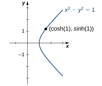
But why are these functions called hyperbolic functions? To answer this question, consider the quantity  . Using the definition of
  and
and  , we see that
 .
.This identity is the analog of the trigonometric identity  . Here, given a value , the point
  lies on the unit hyperbola
  ((Figure)).
 .
.Graphs of Hyperbolic Functions
To graph  and
and  , we make use of the fact that both functions approach
  as , since
  as . As
  approaches
  , whereas approaches
  . Therefore, using the graphs of
  , and
, and  as guides, we graph and . To graph
  , we use the fact that
  for all
  as , and
  as . The graphs of the other three hyperbolic functions can be sketched using the graphs of
  , and ((Figure)).
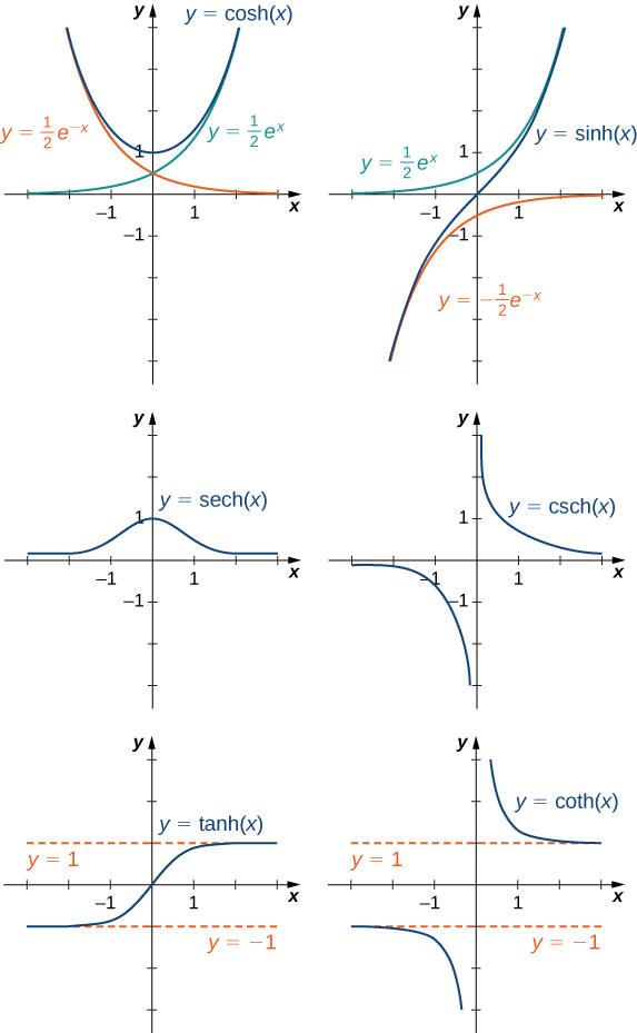 and .
and .Identities Involving Hyperbolic Functions
The identity , shown in (Figure), is one of several identities involving the hyperbolic functions, some of which are listed next. The first four properties follow easily from the definitions of hyperbolic sine and hyperbolic cosine. Except for some differences in signs, most of these properties are analogous to identities for trigonometric functions.
Rule: Identities Involving Hyperbolic Functions


Evaluating Hyperbolic Functions
- Simplify
 .
. - If
 , find the values of the remaining five hyperbolic functions.
Solution
- Using the definition of the function, we write
 .
. - Using the identity
 , we see that
 .
.Since
 for all , we must have
  . Then, using the definitions for the other hyperbolic functions, we conclude that
  , and
, and  .
.
Simplify  .
.
Solution

Hint
Use the definition of the cosh function and the power property of logarithm functions.
Inverse Hyperbolic Functions
From the graphs of the hyperbolic functions, we see that all of them are one-to-one except and  . If we restrict the domains of these two functions to the interval
  , then all the hyperbolic functions are one-to-one, and we can define the inverse hyperbolic functions. Since the hyperbolic functions themselves involve exponential functions, the inverse hyperbolic functions involve logarithmic functions.
Definition
Inverse Hyperbolic Functions

Let’s look at how to derive the first equation. The others follow similarly. Suppose  . Then,
  and, by the definition of the hyperbolic sine function,
  . Therefore,
 .
.Multiplying this equation by  , we obtain
 .
.This can be solved like a quadratic equation, with the solution
 .
.Since  , the only solution is the one with the positive sign. Applying the natural logarithm to both sides of the equation, we conclude that
 .
.Evaluating Inverse Hyperbolic Functions
Evaluate each of the following expressions.


Solution


Evaluate  .
.
Solution
 .
.
Hint
Use the definition of  and simplify.
Key Concepts
- The exponential function is increasing if and decreasing if . Its domain is and its range is .
- The logarithmic function
 is the inverse of . Its domain is and its range is
  .
. - The natural exponential function is and the natural logarithmic function is
 .
. - Given an exponential function or logarithmic function in base , we can make a change of base to convert this function to any base . We typically convert to base .
- The hyperbolic functions involve combinations of the exponential functions and . As a result, the inverse hyperbolic functions involve the natural logarithm.
For the following exercises, evaluate the given exponential functions as indicated, accurate to two significant digits after the decimal.
1.  a.
a.  b.
b.  c.
c. 
Solution
a. 125 b. 2.24 c. 9.74
2.  a.
a.  b.
b.  c.
c. 
3.  a.
a.  b. c.
b. c. 
Solution
a. 0.01 b. 10,000 c. 46.42
4. a.  b.
b.  c.
c. 
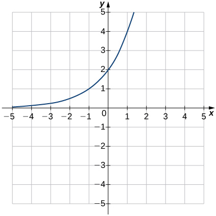
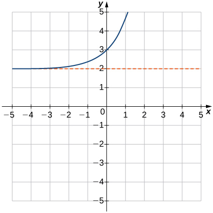
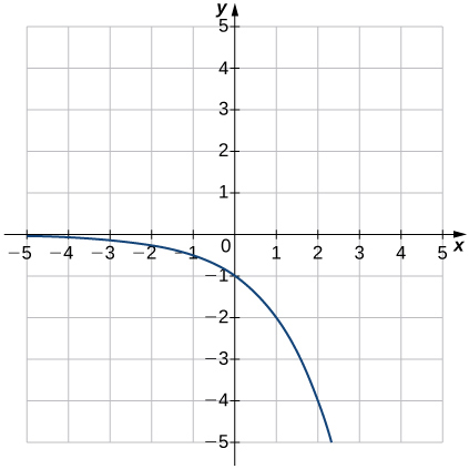
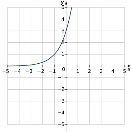
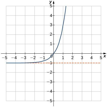
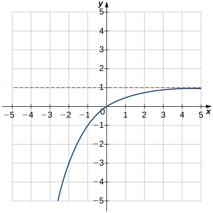
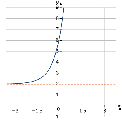
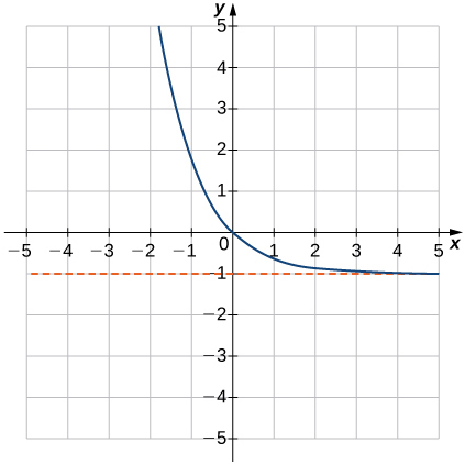
For the following exercises, match the exponential equation to the correct graph.


Solution
d
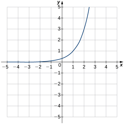
Solution
b
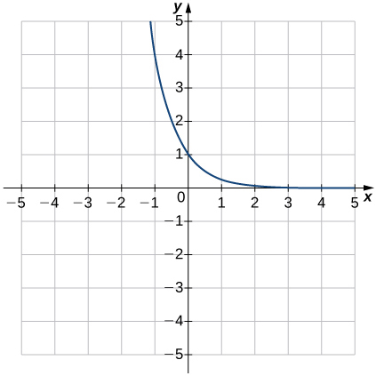
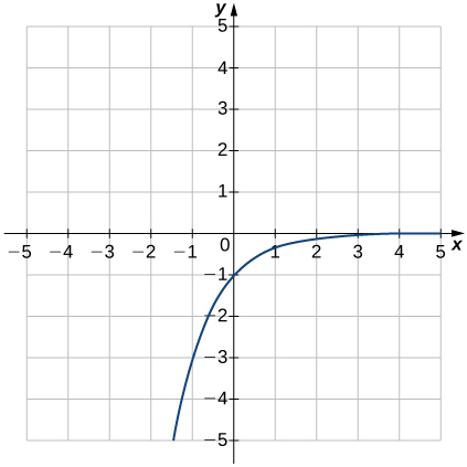
Solution
e
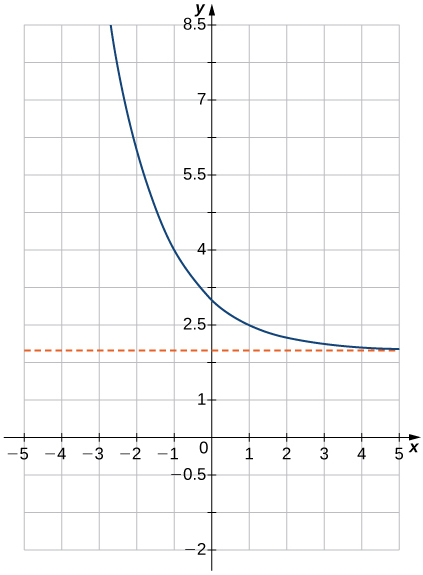
For the following exercises, sketch the graph of the exponential function. Determine the domain, range, and horizontal asymptote.
11. 
Solution
Domain: all real numbers, Range:  , Horizontal asymptote at
12. 
13. 
Solution
Domain: all real numbers, Range: , Horizontal asymptote at
14. 
15. 
Solution
Domain: all real numbers, Range:  , Horizontal asymptote at
16. 
17. 
Solution
Domain: all real numbers, Range:  , Horizontal asymptote at
For the following exercises, write the equation in equivalent exponential form.
18. 
19. 
Solution

20. 
21. 
Solution

22. 
23. 
Solution

24. 
25. 
Solution

For the following exercises, write the equation in equivalent logarithmic form.
26. 
27. 
Solution

28. 
29. 
Solution

30. 
31. ![\sqrt[3]{64}=4](https://ecampusontario.pressbooks.pub/app/uploads/quicklatex/quicklatex.com-93fffb10b8e82aa7182af8790f3c890b_l3.png "Rendered by QuickLaTeX.com")
Solution

32. 
33. 
Solution

34. 
35. 
Solution

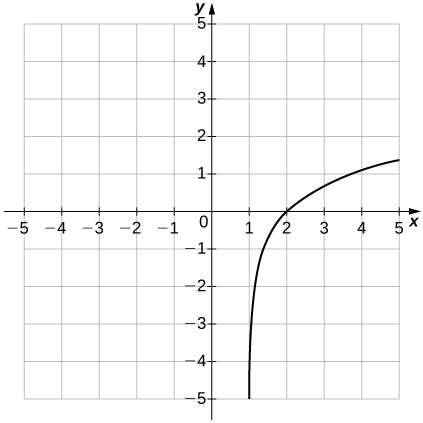
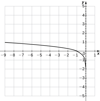
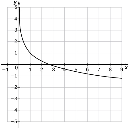
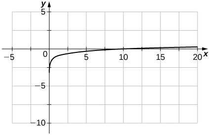
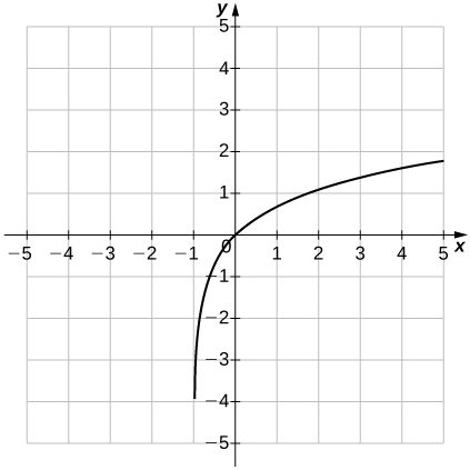
For the following exercises, use the given graphs of the logarithmic functions to determine their domain, range, and vertical asymptote.
36. 
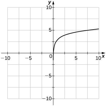
37. 
Solution
Domain:  Range: , Vertical asymptote at
38. 
39. 
Solution
Domain: , Range: , Vertical asymptote at
40. 
41. 
Solution
Domain:  , Range: , Vertical asymptote at
For the following exercises, use properties of logarithms to write the expressions as a sum, difference, and/or product of logarithms.
42. 
43. 
Solution

44. ![\ln a\sqrt[3]{b}](https://ecampusontario.pressbooks.pub/app/uploads/quicklatex/quicklatex.com-5cf03bd49a690140afbd733e43cd9664_l3.png "Rendered by QuickLaTeX.com")
45. 
Solution

46. ![\log_4 \frac{\sqrt[3]{xy}}{64}](https://ecampusontario.pressbooks.pub/app/uploads/quicklatex/quicklatex.com-295a2b2cd0add17fee7b504d7ad5c49d_l3.png "Rendered by QuickLaTeX.com")
47. 
Solution

For the following exercises, solve the exponential equation exactly.
48. 
49. 
Solution

50. 
51. 
Solution

52. 
53. 
Solution

54. 
55. 
Solution

For the following exercises, solve the logarithmic equation exactly, if possible.
56. 
57. 
Solution

58. 
59. 
Solution
60. 
61. 
Solution
62. 
63. 
Solution

For the following exercises, use the change-of-base formula and either base 10 or base to evaluate the given expressions. Answer in exact form and in approximate form, rounding to four decimal places.
64. 
65. 
Solution

66. 
67. 
Solution

68. 
69. 
Solution

70. Rewrite the following expressions in terms of exponentials and simplify.
a. 
b. 
c. 
d. 
71. [T] The number of bacteria  in a culture after days can be modeled by the function
  . Find the number of bacteria present after 15 days.
Solution

72. [T] The demand  (in millions of barrels) for oil in an oil-rich country is given by the function
  , where is the price (in dollars) of a barrel of oil. Find the amount of oil demanded (to the nearest million barrels) when the price is between $15 and $20.
73. [T] The accumulated amount  of a $100,000 investment whose interest compounds continuously for years is given by
  . Find the amount accumulated in 5 years.
Solution
Approximately $131,653 is accumulated in 5 years.
74. [T] An investment is compounded monthly, quarterly, or yearly and is given by the function  , where is the value of the investment at time
  is the initial principle that was invested,
  is the annual interest rate, and is the number of time the interest is compounded per year. Given a yearly interest rate of 3.5% and an initial principle of $100,000, find the amount accumulated in 5 years for interest that is compounded a. daily, b., monthly, c. quarterly, and d. yearly.
75. [T] The concentration of hydrogen ions in a substance is denoted by ![[\text{H}^{+}]](https://ecampusontario.pressbooks.pub/app/uploads/quicklatex/quicklatex.com-81edbfd2c8045816664d059f9829f2aa_l3.png "Rendered by QuickLaTeX.com") , measured in moles per liter. The pH of a substance is defined by the logarithmic function
, measured in moles per liter. The pH of a substance is defined by the logarithmic function ![\text{pH}=−\log[\text{H}^{+}]](https://ecampusontario.pressbooks.pub/app/uploads/quicklatex/quicklatex.com-c333e3c722d7fa9f4174c45ed8a6707d_l3.png "Rendered by QuickLaTeX.com") . This function is used to measure the acidity of a substance. The pH of water is 7. A substance with a pH less than 7 is an acid, whereas one that has a pH of more than 7 is a base.
. This function is used to measure the acidity of a substance. The pH of water is 7. A substance with a pH less than 7 is an acid, whereas one that has a pH of more than 7 is a base.
- Find the pH of the following substances. Round answers to one digit.
- Determine whether the substance is an acid or a base.
- Eggs:
![[\text{H}^{+}]=1.6 \times 10^{-8}](https://ecampusontario.pressbooks.pub/app/uploads/quicklatex/quicklatex.com-a9cf99af68ad37d9f6bd4de495350d74_l3.png "Rendered by QuickLaTeX.com") mol/L
mol/L - Beer:
![[\text{H}^{+}]=3.16 \times 10^{-3}](https://ecampusontario.pressbooks.pub/app/uploads/quicklatex/quicklatex.com-26442820e092e0e35b4b592329c4842b_l3.png "Rendered by QuickLaTeX.com") mol/L
mol/L - Tomato Juice:
![[\text{H}^{+}]=7.94 \times 10^{-5}](https://ecampusontario.pressbooks.pub/app/uploads/quicklatex/quicklatex.com-7f920f9db6486117648814afc1a9fdc5_l3.png "Rendered by QuickLaTeX.com") mol/L
mol/L
- Eggs:
Solution
i. a. pH = 8 b. Base ii. a. pH = 3 b. Acid iii. a. pH = 4 b. Acid
76. [T] Iodine-131 is a radioactive substance that decays according to the function  , where
  is the initial quantity of a sample of the substance and is in days. Determine how long it takes (to the nearest day) for 95% of a quantity to decay.
77. [T] According to the World Bank, at the end of 2013 (  ) the U.S. population was 316 million and was increasing according to the following model:
 ,
,
where is measured in millions of people and is measured in years after 2013.
- Based on this model, what will be the population of the United States in 2020?
- Determine when the U.S. population will be twice what it is in 2013.
Solution
a.  million b. 94 years from 2013, or in 2107
78. [T] The amount accumulated after 1000 dollars is invested for years at an interest rate of 4% is modeled by the function  .
.
- Find the amount accumulated after 5 years and 10 years.
- Determine how long it takes for the original investment to triple.
79. [T] A bacterial colony grown in a lab is known to double in number in 12 hours. Suppose, initially, there are 1000 bacteria present.
- Use the exponential function
 to determine the value
  , which is the growth rate of the bacteria. Round to four decimal places.
 - Determine approximately how long it takes for 200,000 bacteria to grow.
Solution
a.  b.
b.  hours
hours
80. [T] The rabbit population on a game reserve doubles every 6 months. Suppose there were 120 rabbits initially.
- Use the exponential function
 to determine the growth rate constant . Round to four decimal places.
 - Use the function in part a. to determine approximately how long it takes for the rabbit population to reach 3500.
81. [T] The 1906 earthquake in San Francisco had a magnitude of 8.3 on the Richter scale. At the same time, in Japan, an earthquake with magnitude 4.9 caused only minor damage. Approximately how much more energy was released by the San Francisco earthquake than by the Japanese earthquake?
Solution
The San Francisco earthquake had  or
or  times more energy than the Japan earthquake.
Glossary
- base
- the number in the exponential function and the logarithmic function

- exponent
- the value in the expression
- hyperbolic functions
- the functions denoted
 , and
, and  , which involve certain combinations of and
- inverse hyperbolic functions
- the inverses of the hyperbolic functions where and
 are restricted to the domain ; each of these functions can be expressed in terms of a composition of the natural logarithm function and an algebraic function
- natural exponential function
- the function
- natural logarithm
- the function

- number e
- as
 gets larger, the quantity
  gets closer to some real number; we define that real number to be ; the value of is approximately 2.718282

Hint