Chapter 2.3: Basic Classes of Functions
Learning Objectives
- Calculate the slope of a linear function and interpret its meaning.
- Recognize the degree of a polynomial.
- Find the roots of a quadratic polynomial.
- Describe the graphs of basic odd and even polynomial functions.
- Identify a rational function.
- Describe the graphs of power and root functions.
- Explain the difference between algebraic and transcendental functions.
- Graph a piecewise-defined function.
- Sketch the graph of a function that has been shifted, stretched, or reflected from its initial graph position.
We have studied the general characteristics of functions, so now let’s examine some specific classes of functions. We begin by reviewing the basic properties of linear and quadratic functions, and then generalize to include higher-degree polynomials. By combining root functions with polynomials, we can define general algebraic functions and distinguish them from the transcendental functions we examine later in this chapter. We finish the section with examples of piecewise-defined functions and take a look at how to sketch the graph of a function that has been shifted, stretched, or reflected from its initial form.
Linear Functions and Slope
The easiest type of function to consider is a linear function. Linear functions have the form  , where
  and
and  are constants. In (Figure), we see examples of linear functions when is positive, negative, and zero. Note that if
  , the graph of the line rises as
  increases. In other words, is increasing on
  . If
. If  , the graph of the line falls as increases. In this case, is decreasing on . If
  , the line is horizontal.
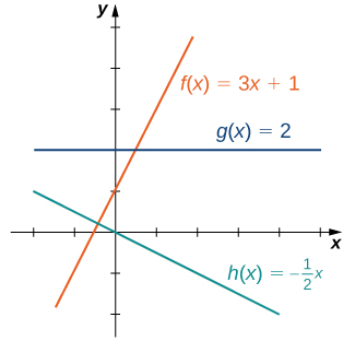
 and one function is a horizontal line.
As suggested by (Figure), the graph of any linear function is a line. One of the distinguishing features of a line is its slope. The slope is the change in  for each unit change in . The slope measures both the steepness and the direction of a line. If the slope is positive, the line points upward when moving from left to right. If the slope is negative, the line points downward when moving from left to right. If the slope is zero, the line is horizontal. To calculate the slope of a line, we need to determine the ratio of the change in versus the change in . To do so, we choose any two points
  and
and  on the line and calculate
  . In (Figure), we see this ratio is independent of the points chosen.
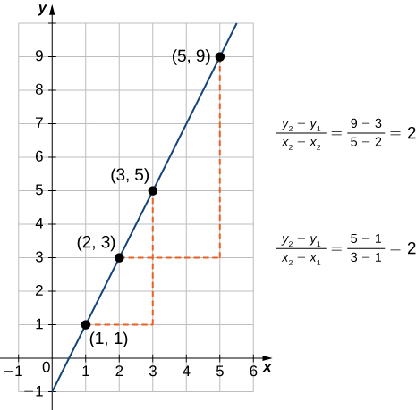
 is independent of the choice of points and on the line.
Definition
Consider line  passing through points and . Let
  and
and  denote the changes in and , respectively. The slope of the line is
 .
.We now examine the relationship between slope and the formula for a linear function. Consider the linear function given by the formula . As discussed earlier, we know the graph of a linear function is given by a line. We can use our definition of slope to calculate the slope of this line. As shown, we can determine the slope by calculating for any points and on the line. Evaluating the function  at
at  , we see that
  is a point on this line. Evaluating this function at
  , we see that
  is also a point on this line. Therefore, the slope of this line is
 .
.We have shown that the coefficient is the slope of the line. We can conclude that the formula describes a line with slope . Furthermore, because this line intersects the -axis at the point , we see that the -intercept for this linear function is . We conclude that the formula tells us the slope, , and the -intercept, , for this line. Since we often use the symbol  to denote the slope of a line, we can write

to denote the slope-intercept form of a linear function.
Sometimes it is convenient to express a linear function in different ways. For example, suppose the graph of a linear function passes through the point and the slope of the line is . Since any other point  on the graph of must satisfy the equation
 ,
,this linear function can be expressed by writing
 .
.We call this equation the point-slope equation for that linear function.
Since every nonvertical line is the graph of a linear function, the points on a nonvertical line can be described using the slope-intercept or point-slope equations. However, a vertical line does not represent the graph of a function and cannot be expressed in either of these forms. Instead, a vertical line is described by the equation  for some constant
  . Since neither the slope-intercept form nor the point-slope form allows for vertical lines, we use the notation
 ,
,where  are both not zero, to denote the standard form of a line.
Definition
Consider a line passing through the point with slope . The equation

is the point-slope equation for that line.
Consider a line with slope and -intercept . The equation

is an equation for that line in slope-intercept form.
The standard form of a line is given by the equation
,where and are both not zero. This form is more general because it allows for a vertical line, .
Finding the Slope and Equations of Lines
Consider the line passing through the points  and
and  , as shown in (Figure).
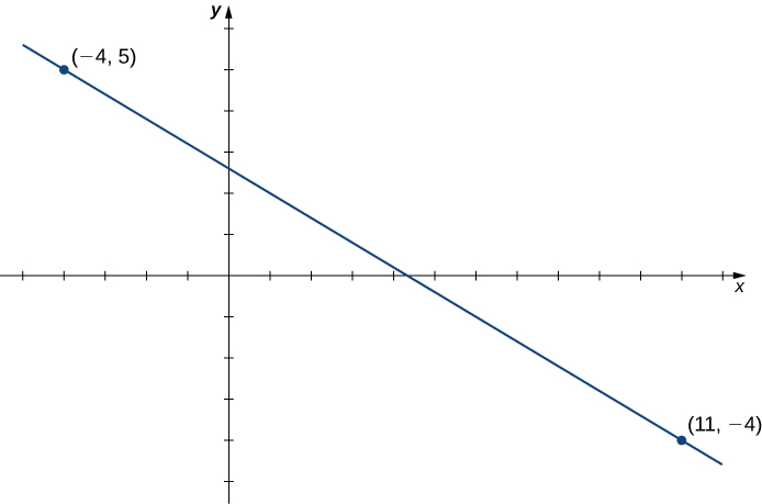
- Find the slope of the line.
- Find an equation for this linear function in point-slope form.
- Find an equation for this linear function in slope-intercept form.
Solution
- The slope of the line is
 .
. - To find an equation for the linear function in point-slope form, use the slope
 and choose any point on the line. If we choose the point , we get the equation
 .
. - To find an equation for the linear function in slope-intercept form, solve the equation in part b. for
 . When we do this, we get the equation
 .
.
Consider the line passing through points  and
and  . Find the slope of the line.
Find an equation of that line in point-slope form. Find an equation of that line in slope-intercept form.
Solution
 . The point-slope form is
 .
.
The slope-intercept form is
 .
.
A Linear Distance Function
Jessica leaves her house at 5:50 a.m. and goes for a 9-mile run. She returns to her house at 7:08 a.m. Answer the following questions, assuming Jessica runs at a constant pace.
- Describe the distance
 (in miles) Jessica runs as a linear function of her run time
  (in minutes).
 - Sketch a graph of .
- Interpret the meaning of the slope.
Solution
- At time
 , Jessica is at her house, so
  . At time
  minutes, Jessica has finished running 9 mi, so
  . The slope of the linear function is
 .
.The
-intercept is  , so the equation for this linear function is
 .
. - To graph , use the fact that the graph passes through the origin and has slope
 .
.
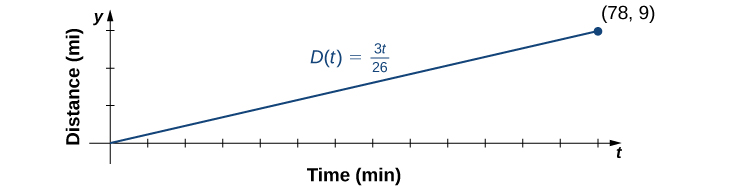
- The slope
 describes the distance (in miles) Jessica runs per minute, or her average velocity.
Polynomials
A linear function is a special type of a more general class of functions: polynomials. A polynomial function is any function that can be written in the form

for some integer  and constants
  , where
  . In the case when
  , we allow for
  ; if , the function
  is called the zero function. The value
  is called the degree of the polynomial; the constant
  is called the leading coefficient. A linear function of the form is a polynomial of degree 1 if
  and degree 0 if
  . A polynomial of degree 0 is also called a constant function. A polynomial function of degree 2 is called a quadratic function. In particular, a quadratic function has the form
  , where
  . A polynomial function of degree 3 is called a cubic function.
Power Functions
Some polynomial functions are power functions. A power function is any function of the form  , where and are any real numbers. The exponent in a power function can be any real number, but here we consider the case when the exponent is a positive integer. (We consider other cases later.) If the exponent is a positive integer, then
  is a polynomial. If is even, then is an even function because
  if is even. If is odd, then is an odd function because
  if is odd ((Figure)).
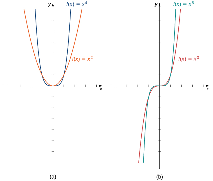
 is an even function. (b) For any odd integer is an odd function.
Behavior at Infinity
To determine the behavior of a function as the inputs approach infinity, we look at the values as the inputs, , become larger. For some functions, the values of approach a finite number. For example, for the function  , the values
  become closer and closer to zero for all values of as they get larger and larger. For this function, we say ” approaches two as goes to infinity,” and we write
  as
as  . The line
  is a horizontal asymptote for the function because the graph of the function gets closer to the line as gets larger.
For other functions, the values may not approach a finite number but instead may become larger for all values of as they get larger. In that case, we say ” approaches infinity as approaches infinity,” and we write  as . For example, for the function
  , the outputs become larger as the inputs get larger. We can conclude that the function approaches infinity as approaches infinity, and we write
  as . The behavior as
  and the meaning of
  as
as  or can be defined similarly. We can describe what happens to the values of as and as as the end behavior of the function.
To understand the end behavior for polynomial functions, we can focus on quadratic and cubic functions. The behavior for higher-degree polynomials can be analyzed similarly. Consider a quadratic function . If , the values  as
as  . If , the values
  as . Since the graph of a quadratic function is a parabola, the parabola opens upward if ; the parabola opens downward if . (See (Figure)(a).)
Now consider a cubic function  . If , then as and
  as
as  . If , then as and as . As we can see from both of these graphs, the leading term of the polynomial determines the end behavior. (See (Figure)(b).)
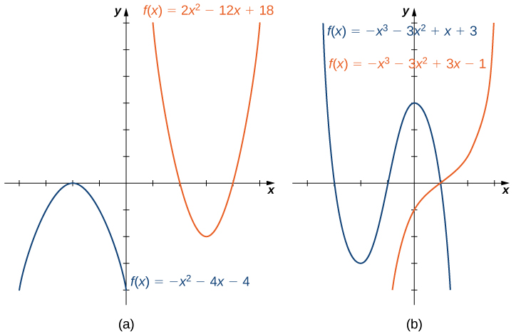 , the parabola opens upward. If , the parabola opens downward. (b) For a cubic function , if the leading coefficient , the values as
  and the values
  as . If the leading coefficient , the opposite is true.
Zeros of Polynomial Functions
Another characteristic of the graph of a polynomial function is where it intersects the -axis. To determine where a function intersects the -axis, we need to solve the equation for . In the case of the linear function , the -intercept is given by solving the equation  . In this case, we see that the -intercept is given by
  . In the case of a quadratic function, finding the -intercept(s) requires finding the zeros of a quadratic equation:
  . In some cases, it is easy to factor the polynomial
  to find the zeros. If not, we make use of the quadratic formula.
Rule: The Quadratic Formula
Consider the quadratic equation
,where . The solutions of this equation are given by the quadratic formula
 .
.If the discriminant  , this formula tells us there are two real numbers that satisfy the quadratic equation. If
  , this formula tells us there is only one solution, and it is a real number. If
  , no real numbers satisfy the quadratic equation.
In the case of higher-degree polynomials, it may be more complicated to determine where the graph intersects the -axis. In some instances, it is possible to find the -intercepts by factoring the polynomial to find its zeros. In other cases, it is impossible to calculate the exact values of the -intercepts. However, as we see later in the text, in cases such as this, we can use analytical tools to approximate (to a very high degree) where the -intercepts are located. Here we focus on the graphs of polynomials for which we can calculate their zeros explicitly.
Graphing Polynomial Functions
For the following functions a. and b., i. describe the behavior of as , ii. find all zeros of , and iii. sketch a graph of .
Solution
- The function
 is a quadratic function.
- Because
 , as
, as  .
. - To find the zeros of , use the quadratic formula. The zeros are
 .
. - To sketch the graph of , use the information from your previous answers and combine it with the fact that the graph is a parabola opening downward.
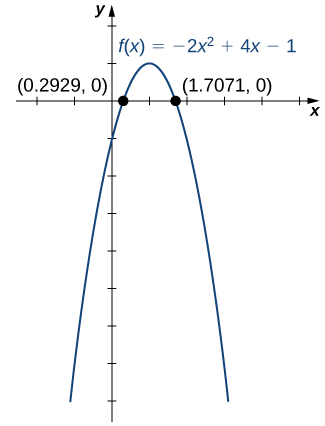
- Because
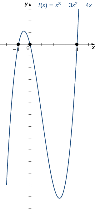
- The function
 is a cubic function.
- Because
 , as
, as  . As
. As  .
. - To find the zeros of , we need to factor the polynomial. First, when we factor out of all the terms, we find
 .
.Then, when we factor the quadratic function
 , we find
 .
.Therefore, the zeros of
are  .
. - Combining the results from parts i. and ii., draw a rough sketch of .
- Because
Consider the quadratic function  . Find the zeros of . Does the parabola open upward or downward?
Solution
The zeros are  . The parabola opens upward.
Hint
Use the quadratic formula.
Mathematical Models
A large variety of real-world situations can be described using mathematical models. A mathematical model is a method of simulating real-life situations with mathematical equations. Physicists, engineers, economists, and other researchers develop models by combining observation with quantitative data to develop equations, functions, graphs, and other mathematical tools to describe the behavior of various systems accurately. Models are useful because they help predict future outcomes. Examples of mathematical models include the study of population dynamics, investigations of weather patterns, and predictions of product sales.
As an example, let’s consider a mathematical model that a company could use to describe its revenue for the sale of a particular item. The amount of revenue  a company receives for the sale of items sold at a price of
  dollars per item is described by the equation
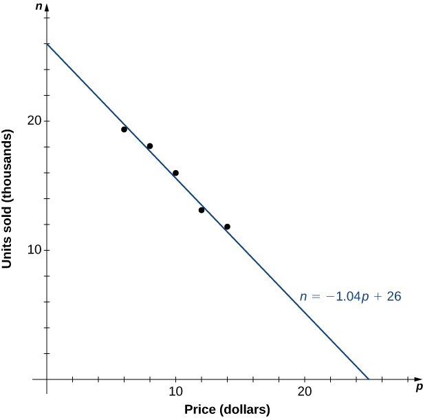
  . The company is interested in how the sales change as the price of the item changes. Suppose the data in (Figure) show the number of units a company sells as a function of the price per item.
 |
6 | 8 | 10 | 12 | 14 |
 |
19.4 | 18.5 | 16.2 | 13.8 | 12.2 |
In (Figure), we see the graph the number of units sold (in thousands) as a function of price (in dollars). We note from the shape of the graph that the number of units sold is likely a linear function of price per item, and the data can be closely approximated by the linear function  for
for  , where predicts the number of units sold in thousands. Using this linear function, the revenue (in thousands of dollars) can be estimated by the quadratic function

for . In Example, we use this quadratic function to predict the amount of revenue the company receives depending on the price the company charges per item. Note that we cannot conclude definitively the actual number of units sold for values of , for which no data are collected. However, given the other data values and the graph shown, it seems reasonable that the number of units sold (in thousands) if the price charged is dollars may be close to the values predicted by the linear function .
 to estimate this function.
Maximizing Revenue
A company is interested in predicting the amount of revenue it will receive depending on the price it charges for a particular item. Using the data from (Figure), the company arrives at the following quadratic function to model revenue as a function of price per item :
for .
- Predict the revenue if the company sells the item at a price of
 and
and  .
. - Find the zeros of this function and interpret the meaning of the zeros.
- Sketch a graph of .
- Use the graph to determine the value of that maximizes revenue. Find the maximum revenue.
Solution
- Evaluating the revenue function at
 and
and  , we can conclude that
 .
. - The zeros of this function can be found by solving the equation
 . When we factor the quadratic expression, we get
  . The solutions to this equation are given by
  . For these values of , the revenue is zero. When
  , the revenue is zero because the company is giving away its merchandise for free. When
  , the revenue is zero because the price is too high, and no one will buy any items.
 - Knowing the fact that the function is quadratic, we also know the graph is a parabola. Since the leading coefficient is negative, the parabola opens downward. One property of parabolas is that they are symmetric about the axis of symmetry, located at the middle of its graph, so since the zeros are at
 and
and  , the parabola must be symmetric about the line halfway between them, or
  .
.
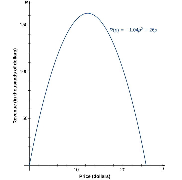
- The function is a parabola with zeros at and , and it is symmetric about the line , so the maximum revenue occurs at a price of
 per item. At that price, the revenue is
  .
.
Algebraic Functions
By allowing for quotients and fractional powers in polynomial functions, we create a larger class of functions. An algebraic function is one that involves addition, subtraction, multiplication, division, rational powers, and roots. Two types of algebraic functions are rational functions and root functions.
Just as rational numbers are quotients of integers, rational functions are quotients of polynomials. In particular, a rational function is any function of the form  , where
  and
and  are polynomials. For example,
 and
and 
are rational functions. A root function is a power function of the form  , where is a positive integer greater than one. For example,
  is the square-root function and
 ![g(x)=x^{1/3}=\sqrt[3]{x}](https://ecampusontario.pressbooks.pub/app/uploads/quicklatex/quicklatex.com-3067c00e6edf7056da3c3723c99d8ec2_l3.png "Rendered by QuickLaTeX.com") is the cube-root function. By allowing for compositions of root functions and rational functions, we can create other algebraic functions. For example,
is the cube-root function. By allowing for compositions of root functions and rational functions, we can create other algebraic functions. For example,  is an algebraic function.
Finding Domain and Range for Algebraic Functions
For each of the following functions, find the domain and range.
Solution
- It is not possible to divide by zero, so the domain is the set of real numbers such that
 . To find the range, we need to find the values for which there exists a real number such that
 .
.When we multiply both sides of this equation by
 , we see that must satisfy the equation
 .
.From this equation, we can see that
must satisfy .
.If
 , this equation has no solution. On the other hand, as long as
  ,
,
satisfies this equation. We can conclude that the range of
is  .
. - To find the domain of , we need
 . When we factor, we write
  . This inequality holds if and only if both terms are positive or both terms are negative. For both terms to be positive, we need to find such that
 and
and  .
.These two inequalities reduce to
 and
and  . Therefore, the set
  must be part of the domain. For both terms to be negative, we need
 and .
and .These two inequalities also reduce to
 and . There are no values of that satisfy both of these inequalities. Thus, we can conclude the domain of this function is
  .
.
If , then
  . Therefore,
  , and the range of is
  .
.
Find the domain and range for the function  .
.
Solution
The domain is the set of real numbers such that  . The range is the set
  .
.
Hint
The denominator cannot be zero. Solve the equation  for to find the range.
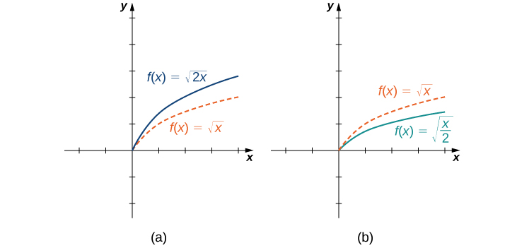
The root functions have defining characteristics depending on whether is odd or even. For all even integers  , the domain of is the interval
  . For all odd integers
  , the domain of is the set of all real numbers. Since
  for odd integers
  is an odd function if is odd. See the graphs of root functions for different values of in (Figure).
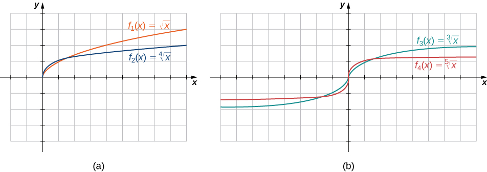 is even, the domain of
 ![f(x)=\sqrt[n]{x}](https://ecampusontario.pressbooks.pub/app/uploads/quicklatex/quicklatex.com-ca6c3302aac609e9214e62444cfec2bb_l3.png "Rendered by QuickLaTeX.com") is . (b) If is odd, the domain of is
is . (b) If is odd, the domain of is  and the function is an odd function.
Finding Domains for Algebraic Functions
For each of the following functions, determine the domain of the function.


![f(x)=\sqrt[3]{2x-1}](https://ecampusontario.pressbooks.pub/app/uploads/quicklatex/quicklatex.com-85a5bc4e38079200edf49dcfdcdba93c_l3.png "Rendered by QuickLaTeX.com")
Solution
- You cannot divide by zero, so the domain is the set of values such that
 . Therefore, the domain is
  .
. - You need to determine the values of for which the denominator is zero. Since
 for all real numbers , the denominator is never zero. Therefore, the domain is .
 - Since the square root of a negative number is not a real number, the domain is the set of values for which
 . Therefore, the domain is
  .
. - The cube root is defined for all real numbers, so the domain is the interval .
Find the domain for each of the following functions:  and
and  .
.
Solution
The domain of is The domain of  is
is  .
.
Hint
Determine the values of when the expression in the denominator of is nonzero, and find the values of when the expression inside the radical of is nonnegative.
Transcendental Functions
Thus far, we have discussed algebraic functions. Some functions, however, cannot be described by basic algebraic operations. These functions are known as transcendental functions because they are said to “transcend,” or go beyond, algebra. The most common transcendental functions are trigonometric, exponential, and logarithmic functions. A trigonometric function relates the ratios of two sides of a right triangle. They are  , and
, and  . (We discuss trigonometric functions later in the chapter.) An exponential function is a function of the form
  , where the base
  . A logarithmic function is a function of the form
  for some constant , where
  if and only if
  . (We also discuss exponential and logarithmic functions later in the chapter.)
Classifying Algebraic and Transcendental Functions
Classify each of the following functions, a. through c., as algebraic or transcendental.


Solution
- Since this function involves basic algebraic operations only, it is an algebraic function.
- This function cannot be written as a formula that involves only basic algebraic operations, so it is transcendental. (Note that algebraic functions can only have powers that are rational numbers.)
- As in part b., this function cannot be written using a formula involving basic algebraic operations only; therefore, this function is transcendental.
Is  an algebraic or a transcendental function?
Solution
Algebraic
Piecewise-Defined Functions
Sometimes a function is defined by different formulas on different parts of its domain. A function with this property is known as a piecewise-defined function. The absolute value function is an example of a piecewise-defined function because the formula changes with the sign of :
 .
.Other piecewise-defined functions may be represented by completely different formulas, depending on the part of the domain in which a point falls. To graph a piecewise-defined function, we graph each part of the function in its respective domain, on the same coordinate system. If the formula for a function is different for  and
and  , we need to pay special attention to what happens at
  when we graph the function. Sometimes the graph needs to include an open or closed circle to indicate the value of the function at . We examine this in the next example.
Graphing a Piecewise-Defined Function
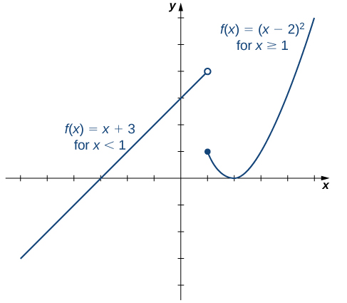
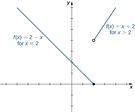
Sketch a graph of the following piecewise-defined function:

Solution
Graph the linear function  on the interval
  and graph the quadratic function
  on the interval
  . Since the value of the function at is given by the formula
  , we see that
  . To indicate this on the graph, we draw a closed circle at the point
  . The value of the function is given by
  for all
  , but not at . To indicate this on the graph, we draw an open circle at .
and quadratic for  .
.Sketch a graph of the function

Solution
Hint
Graph one linear function for  and then graph a different linear function for
  .
.
Parking Fees Described by a Piecewise-Defined Function
In a big city, drivers are charged variable rates for parking in a parking garage. They are charged $10 for the first hour or any part of the first hour and an additional $2 for each hour or part thereof up to a maximum of $30 for the day. The parking garage is open from 6 a.m. to 12 midnight.
- Write a piecewise-defined function that describes the cost
 to park in the parking garage as a function of hours parked .
 - Sketch a graph of this function
 .
.
Solution
- Since the parking garage is open 18 hours each day, the domain for this function is
 . The cost to park a car at this parking garage can be described piecewise by the function

- The graph of the function consists of several horizontal line segments.

The cost of mailing a letter is a function of the weight of the letter. Suppose the cost of mailing a letter is  for the first ounce and
  for each additional ounce. Write a piecewise-defined function describing the cost as a function of the weight for
  , where is measured in cents and is measured in ounces.
Solution

Hint
The piecewise-defined function is constant on the intervals ![(0,1], \, (1,2], \, \cdots](https://ecampusontario.pressbooks.pub/app/uploads/quicklatex/quicklatex.com-4d3a006f84ae1660e2066345a862ca29_l3.png "Rendered by QuickLaTeX.com")
Transformations of Functions
We have seen several cases in which we have added, subtracted, or multiplied constants to form variations of simple functions. In the previous example, for instance, we subtracted 2 from the argument of the function  to get the function . This subtraction represents a shift of the function two units to the right. A shift, horizontally or vertically, is a type of transformation of a function. Other transformations include horizontal and vertical scalings, and reflections about the axes.
A vertical shift of a function occurs if we add or subtract the same constant to each output . For  , the graph of
  is a shift of the graph of up
  units, whereas the graph of
  is a shift of the graph of down units. For example, the graph of the function
  is the graph of
  shifted up 4 units; the graph of the function
  is the graph of shifted down 4 units ((Figure)).
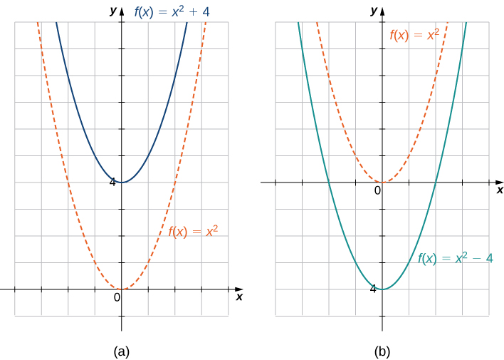 , the graph of
  is a vertical shift up units of the graph of
  . (b) For , the graph of
  is a vertical shift down units of the graph of .
A horizontal shift of a function occurs if we add or subtract the same constant to each input . For , the graph of  is a shift of the graph of to the left units; the graph of
  is a shift of the graph of to the right units. Why does the graph shift left when adding a constant and shift right when subtracting a constant? To answer this question, let’s look at an example.
Consider the function  and evaluate this function at
  Since
Since  and
and  , the graph of is the graph of
  shifted left 3 units. Similarly, the graph of
  is the graph of shifted right 3 units ((Figure)).
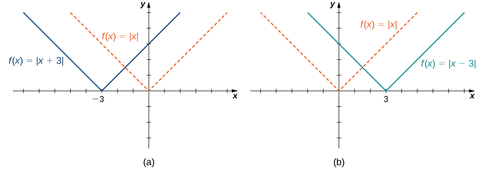 , the graph of
  is a horizontal shift left units of the graph of . (b) For , the graph of
  is a horizontal shift right units of the graph of .
A vertical scaling of a graph occurs if we multiply all outputs of a function by the same positive constant. For , the graph of the function  is the graph of scaled vertically by a factor of . If
  , the values of the outputs for the function are larger than the values of the outputs for the function ; therefore, the graph has been stretched vertically. If
  , then the outputs of the function are smaller, so the graph has been compressed. For example, the graph of the function is the graph of stretched vertically by a factor of 3, whereas the graph of
  is the graph of compressed vertically by a factor of 3 ((Figure)).
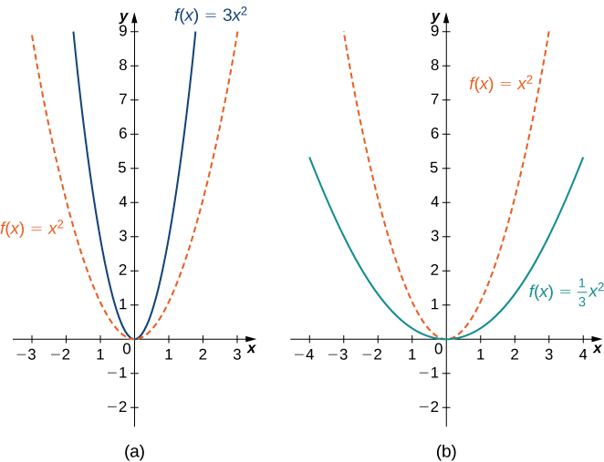 , the graph of
  is a vertical stretch of the graph of . (b) If , the graph of is a vertical compression of the graph of .
The horizontal scaling of a function occurs if we multiply the inputs by the same positive constant. For , the graph of the function  is the graph of scaled horizontally by a factor of . If , the graph of is the graph of compressed horizontally. If , the graph of is the graph of stretched horizontally. For example, consider the function
  and evaluate at
  Since
Since  , the graph of is the graph of
  compressed horizontally. The graph of
  is a horizontal stretch of the graph of ((Figure)).
 , the graph of
  is a horizontal compression of the graph of . (b) If , the graph of is a horizontal stretch of the graph of .
We have explored what happens to the graph of a function when we multiply by a constant to get a new function . We have also discussed what happens to the graph of a function when we multiply the independent variable by to get a new function . However, we have not addressed what happens to the graph of the function if the constant is negative. If we have a constant  , we can write as a positive number multiplied by -1; but, what kind of transformation do we get when we multiply the function or its argument by -1? When we multiply all the outputs by -1, we get a reflection about the -axis. When we multiply all inputs by -1, we get a reflection about the -axis. For example, the graph of
  is the graph of
  reflected about the -axis. The graph of
  is the graph of
  reflected about the -axis ((Figure)).
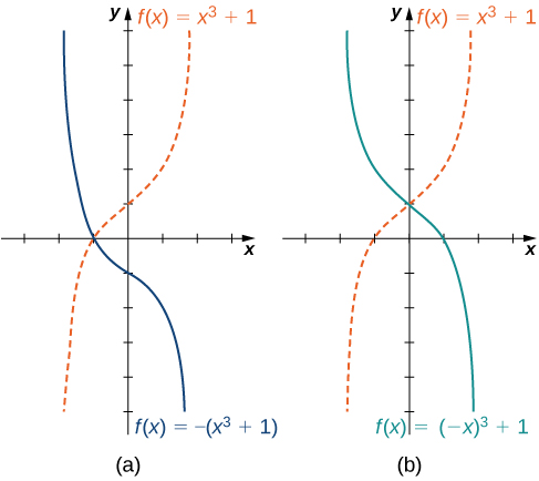
 is the graph of reflected about the -axis. (b) The graph of
  is the graph of reflected about the -axis.
If the graph of a function consists of more than one transformation of another graph, it is important to transform the graph in the correct order. Given a function , the graph of the related function  can be obtained from the graph of by performing the transformations in the following order.
- Horizontal shift of the graph of . If
 , shift left. If
  , shift right.
 - Horizontal scaling of the graph of
 by a factor of
  . If , reflect the graph about the -axis.
 - Vertical scaling of the graph of
 by a factor of
  . If , reflect the graph about the -axis.
 - Vertical shift of the graph of
 . If
. If  , shift up. If
  , shift down.
We can summarize the different transformations and their related effects on the graph of a function in the following table.
0)” and has the values “f(x) +c; f(x) -c; f(x + c); f(x – c); cf(x); f(cx); -f(x); f(-x)”. The second column is labeled “Effect on the graph of f” and the values are “Vertical shift up c units; Vertical shift down c units; Shift left by c units; Shift right by c units; ‘Vertical stretch if c > 1, Vertical compression is 0 < c < 1′; ‘Horizontal stretch if 0 < c 1′; reflection about the x-axis; reflection about the y-axis”.”>
Transformation of  |
Effect on the graph of |
|---|---|
| |
Vertical shift up units |
| |
Vertical shift down units |
| |
Shift left by units |
| |
Shift right by units |
| |
Vertical stretch if ; vertical compression if |
| |
Horizontal stretch if ; horizontal compression if |
 |
Reflection about the -axis |
 |
Reflection about the -axis |
Transforming a Function
For each of the following functions, a. and b., sketch a graph by using a sequence of transformations of a well-known function.
Solution
- Starting with the graph of , shift 2 units to the left, reflect about the -axis, and then shift down 3 units.

Figure 13. The function  can be viewed as a sequence of three transformations of the function .
 - Starting with the graph of , reflect about the -axis, stretch the graph vertically by a factor of 3, and move up 1 unit.

Figure 14. The function  can be viewed as a sequence of three transformations of the function .
Describe how the function  can be graphed using the graph of and a sequence of transformations.
Solution
Shift the graph of to the left 1 unit, reflect about the -axis, then shift down 4 units.
Hint
Use (Table).
Key Concepts
- The power function
 is an even function if is even and
  , and it is an odd function if is odd.
 - The root function has the domain
 if is even and the domain if is odd. If is odd, then is an odd function.
 - The domain of the rational function , where and are polynomial functions, is the set of such that
 .
. - Functions that involve the basic operations of addition, subtraction, multiplication, division, and powers are algebraic functions. All other functions are transcendental. Trigonometric, exponential, and logarithmic functions are examples of transcendental functions.
- A polynomial function with degree satisfies
 as . The sign of the output as depends on the sign of the leading coefficient only and on whether is even or odd.
 - Vertical and horizontal shifts, vertical and horizontal scalings, and reflections about the – and -axes are examples of transformations of functions.
Key Equations
- Point-slope equation of a line
- Slope-intercept form of a line
- Standard form of a line
- Polynomial function

For the following exercises, for each pair of points, a. find the slope of the line passing through the points and b. indicate whether the line is increasing, decreasing, horizontal, or vertical.
1.  and
and
Solution
a. −1 b. Decreasing
2.  and
and 
3.  and
and 
Solution
a. 3/4 b. Increasing
4.  and
and 
5.  and
and 
Solution
a. 4/3 b. Increasing
6.  and
and 
7.  and
and
Solution
a. 0 b. Horizontal
8. and 
For the following exercises, write the equation of the line satisfying the given conditions in slope-intercept form.
9. Slope  , passes through
Solution

10. Slope  , passes through
11. Slope  , passes through
Solution

12. Slope  , -intercept
13. Passing through  and
and 
Solution

14. Passing through  and
and 
15. -intercept  and -intercept
Solution

16. -Intercept and -intercept 
For the following exercises, for each linear equation, a. give the slope and -intercept , if any, and b. graph the line.
17. 
Solution
a.  b.
b.

18. 
19. 
Solution
a.  b.
b.

20. 
21. 
Solution
a.  b.
b.

22. 
23. 
Solution
a.  b.
b.

24. 
For the following exercises, for each polynomial, a. find the degree; b. find the zeros, if any; c. find the -intercept(s), if any; d. use the leading coefficient to determine the graph’s end behavior; and e. determine algebraically whether the polynomial is even, odd, or neither.
25. 
Solution
a. 2; b.  ; c. −5; d. Both ends rise; e. Neither
26. 
27. 
Solution
a. 2; b.  ; c. −1; d. Both ends rise; e. Even
28. 
29. 
Solution
a. 3; b. 0,  ; c. 0; d. Left end rises, right end falls; e. Odd
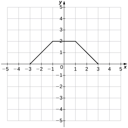
For the following exercises, use the graph of  to graph each transformed function .
30. 
31. 
Solution

For the following exercises, use the graph of  to graph each transformed function .
32. 
33. 
Solution

For the following exercises, use the graph of to graph each transformed function
34. 
35. 
Solution

For the following exercises, for each of the piecewise-defined functions, a. evaluate at the given values of the independent variable and b. sketch the graph.
36.  ;
; 
37.  ;
; 
Solution
a.  b.
b.

38.  ;
; 
39.  ;
; 
Solution
a.  b.
b.

For the following exercises, determine whether the statement is true or false. Explain why.
40.  is a transcendental function.
41. ![g(x)=\sqrt[3]{x}](https://ecampusontario.pressbooks.pub/app/uploads/quicklatex/quicklatex.com-35d87ab6f7e67ac5666e1a707799d67f_l3.png "Rendered by QuickLaTeX.com") is an odd root function
is an odd root function
Solution
True, because 
42. A logarithmic function is an algebraic function.
43. A function of the form  , where is a real valued constant, is an exponential function.
Solution
False, because – where is a real-valued constant – is a power function. Exponential functions are of the form , where is a real-valued constant.
44. The domain of an even root function is all real numbers.
45. [T] A company purchases some computer equipment for $20,500. At the end of a 3-year period, the value of the equipment has decreased linearly to $12,300.
- Find a function
 that determines the value
  of the equipment at the end of years.
 - Find and interpret the meaning of the – and -intercepts for this situation.
- What is the value of the equipment at the end of 5 years?
- When will the value of the equipment be $3000?
Solution
a.  b.
b.  means that the initial purchase price of the equipment is $20,500;
  means that in 7.5 years the computer equipment has no value. c. $6835 d. In approximately 6.4 years
46. [T] Total online shopping during the Christmas holidays has increased dramatically during the past 5 years. In 2012  , total online holiday sales were $42.3 billion, whereas in 2013 they were $48.1 billion.
- Find a linear function
 that estimates the total online holiday sales in the year .
 - Interpret the slope of the graph of .
- Use part a. to predict the year when online shopping during Christmas will reach $60 billion.
47. [T] A family bakery makes cupcakes and sells them at local outdoor festivals. For a music festival, there is a fixed cost of $125 to set up a cupcake stand. The owner estimates that it costs $0.75 to make each cupcake. The owner is interested in determining the total cost as a function of number of cupcakes made.
- Find a linear function that relates cost to , the number of cupcakes made.
- Find the cost to bake 160 cupcakes.
- If the owner sells the cupcakes for $1.50 apiece, how many cupcakes does she need to sell to start making profit? (Hint: Use the INTERSECTION function on a calculator to find this number.)
Solution
a.  b. $245 c. 167 cupcakes
48. [T] A house purchased for $250,000 is expected to be worth twice its purchase price in 18 years.
- Find a linear function that models the price
 of the house versus the number of years since the original purchase.
 - Interpret the slope of the graph of .
- Find the price of the house 15 years from when it was originally purchased.
49. [T] A car was purchased for $26,000. The value of the car depreciates by $1500 per year.
- Find a linear function that models the value of the car after years.
- Find and interpret
 .
.
Solution
a.  b. In 4 years, the value of the car is $20,000.
50. [T] A condominium in an upscale part of the city was purchased for $432,000. In 35 years it is worth $60,500. Find the rate of depreciation.
51. [T] The total cost (in thousands of dollars) to produce a certain item is modeled by the function  , where is the number of items produced. Determine the cost to produce 175 items.
Solution
$30,337.50
52. [T] A professor asks her class to report the amount of time they spent writing two assignments. Most students report that it takes them about 45 minutes to type a four-page assignment and about 1.5 hours to type a nine-page assignment.
- Find the linear function
 that models this situation, where
  is the number of pages typed and is the time in minutes.
 - Use part a. to determine how many pages can be typed in 2 hours.
- Use part a. to determine how long it takes to type a 20-page assignment.
53. [T] The output (as a percent of total capacity) of nuclear power plants in the United States can be modeled by the function  , where is time in years and corresponds to the beginning of 2000. Use the model to predict the percentage output in 2015.
Solution
96% of the total capacity
54. [T] The admissions office at a public university estimates that 65% of the students offered admission to the class of 2019 will actually enroll.
- Find the linear function
 , where is the number of students that actually enroll and is the number of all students offered admission to the class of 2019.
 - If the university wants the 2019 freshman class size to be 1350, determine how many students should be admitted.
Glossary
- algebraic function
- a function involving any combination of only the basic operations of addition, subtraction, multiplication, division, powers, and roots applied to an input variable
- cubic function
- a polynomial of degree 3; that is, a function of the form , where

- degree
- for a polynomial function, the value of the largest exponent of any term
- linear function
- a function that can be written in the form
- logarithmic function
- a function of the form for some base such that
 if and only if
- mathematical model
- A method of simulating real-life situations with mathematical equations
- piecewise-defined function
- a function that is defined differently on different parts of its domain
- point-slope equation
- equation of a linear function indicating its slope and a point on the graph of the function
- polynomial function
- a function of the form
- power function
- a function of the form for any positive integer
- quadratic function
- a polynomial of degree 2; that is, a function of the form where
- rational function
- a function of the form , where and are polynomials
- root function
- a function of the form for any integer
- slope
- the change in for each unit change in
- slope-intercept form
- equation of a linear function indicating its slope and -intercept
- transcendental function
- a function that cannot be expressed by a combination of basic arithmetic operations
- transformation of a function
- a shift, scaling, or reflection of a function

Hint
The slope .
.