Chapter 5.10: Antiderivatives
Learning Objectives
- Find the general antiderivative of a given function.
- Explain the terms and notation used for an indefinite integral.
- State the power rule for integrals.
- Use antidifferentiation to solve simple initial-value problems.
At this point, we have seen how to calculate derivatives of many functions and have been introduced to a variety of their applications. We now ask a question that turns this process around: Given a function  how do we find a function with the derivative
  and why would we be interested in such a function?
We answer the first part of this question by defining antiderivatives. The antiderivative of a function is a function with a derivative  Why are we interested in antiderivatives? The need for antiderivatives arises in many situations, and we look at various examples throughout the remainder of the text. Here we examine one specific example that involves rectilinear motion. In our examination in Derivatives of rectilinear motion, we showed that given a position function
  of an object, then its velocity function
  is the derivative of —that is,
  Furthermore, the acceleration
  is the derivative of the velocity —that is,
  Now suppose we are given an acceleration function
  but not the velocity function
  or the position function
  Since
Since  determining the velocity function requires us to find an antiderivative of the acceleration function. Then, since
  determining the position function requires us to find an antiderivative of the velocity function. Rectilinear motion is just one case in which the need for antiderivatives arises. We will see many more examples throughout the remainder of the text. For now, let’s look at the terminology and notation for antiderivatives, and determine the antiderivatives for several types of functions. We examine various techniques for finding antiderivatives of more complicated functions in the second volume of this text (Introduction to Techniques of Integration).
The Reverse of Differentiation
At this point, we know how to find derivatives of various functions. We now ask the opposite question. Given a function how can we find a function with derivative  If we can find a function
  derivative we call an antiderivative of
Definition
A function is an antiderivative of the function if

for all  in the domain of
Consider the function  Knowing the power rule of differentiation, we conclude that
  is an antiderivative of since
  Are there any other antiderivatives of Yes; since the derivative of any constant
  is zero,
  is also an antiderivative of
  Therefore,
  and
and  are also antiderivatives. Are there any others that are not of the form for some constant
  The answer is no. From Corollary 2 of the Mean Value Theorem, we know that if and
  are differentiable functions such that
  then
then  for some constant
  This fact leads to the following important theorem.
General Form of an Antiderivative
Let be an antiderivative of over an interval  Then,
Then,
- for each constant
 the function
  is also an antiderivative of over
- if is an antiderivative of over
 there is a constant for which
  over
over
In other words, the most general form of the antiderivative of over  is
is 
We use this fact and our knowledge of derivatives to find all the antiderivatives for several functions.
Finding Antiderivatives
For each of the following functions, find all antiderivatives.


Show Answer
a. Because

then  is an antiderivative of
  Therefore, every antiderivative of
  is of the form
  for some constant and every function of the form is an antiderivative of
b. Let  For
For  and
and

For  and
and

Therefore,

Thus,  is an antiderivative of
  Therefore, every antiderivative of
  is of the form
  for some constant and every function of the form is an antiderivative of
c. We have

so  is an antiderivative of
  Therefore, every antiderivative of
  is of the form
  for some constant and every function of the form is an antiderivative of
d. Since

then  is an antiderivative of
  Therefore, every antiderivative of
  is of the form
  for some constant and every function of the form is an antiderivative of
Find all antiderivatives of 
Show Answer

Indefinite Integrals
We now look at the formal notation used to represent antiderivatives and examine some of their properties. These properties allow us to find antiderivatives of more complicated functions. Given a function we use the notation  or
or  to denote the derivative of Here we introduce notation for antiderivatives. If is an antiderivative of we say that is the most general antiderivative of and write

The symbol  is called an integral sign, and
  is called the indefinite integral of
Definition
Given a function the indefinite integral of denoted

is the most general antiderivative of If is an antiderivative of then
The expression  is called the integrand and the variable is the variable of integration.
Given the terminology introduced in this definition, the act of finding the antiderivatives of a function is usually referred to as integrating
For a function and an antiderivative  the functions
  where is any real number, is often referred to as the family of antiderivatives of For example, since
  is an antiderivative of
  and any antiderivative of is of the form
  we write

The collection of all functions of the form where is any real number, is known as the family of antiderivatives of (Figure) shows a graph of this family of antiderivatives.
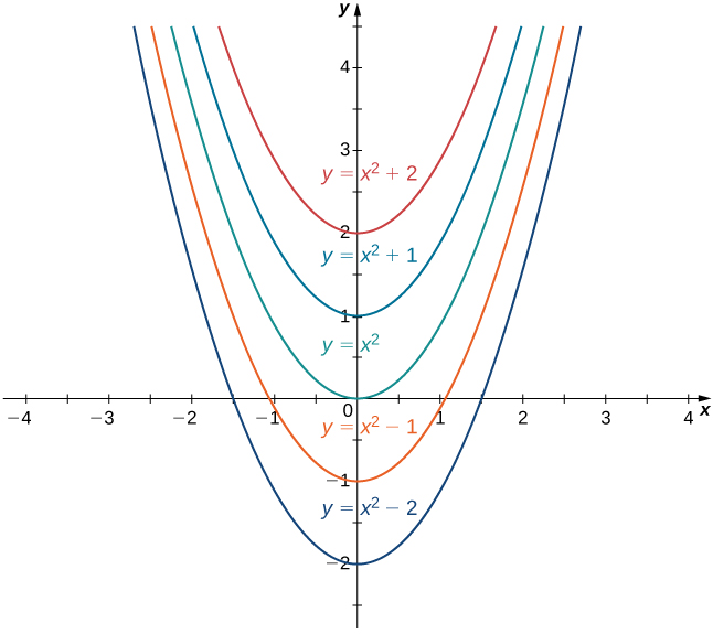 consists of all functions of the form where is any real number.
For some functions, evaluating indefinite integrals follows directly from properties of derivatives. For example, for 

which comes directly from

This fact is known as the power rule for integrals.
Power Rule for Integrals
For

Evaluating indefinite integrals for some other functions is also a straightforward calculation. The following table lists the indefinite integrals for several common functions. A more complete list appears in Appendix B.
| Differentiation Formula | Indefinite Integral |
|---|---|
 |
 |
 |
 for for  |
 |
 |
 |
 |
 |
 |
 |
 |
 |
 |
 |
 |
 |
 |
 |
 |
 |
 |
 |
 |
 |
 |
From the definition of indefinite integral of we know

if and only if is an antiderivative of Therefore, when claiming that
it is important to check whether this statement is correct by verifying that 
Verifying an Indefinite Integral
Each of the following statements is of the form Verify that each statement is correct by showing that
Solution
- Since

the statement

is correct.
Note that we are verifying an indefinite integral for a sum. Furthermore, and are antiderivatives of and
  respectively, and the sum of the antiderivatives is an antiderivative of the sum. We discuss this fact again later in this section.
 - Using the product rule, we see that

Therefore, the statement

is correct.
Note that we are verifying an indefinite integral for a product. The antiderivative is not a product of the antiderivatives. Furthermore, the product of antiderivatives,
  is not an antiderivative of
  since
since
In general, the product of antiderivatives is not an antiderivative of a product.
Verify that 
Solution

Hint
Calculate 
In (Figure), we listed the indefinite integrals for many elementary functions. Let’s now turn our attention to evaluating indefinite integrals for more complicated functions. For example, consider finding an antiderivative of a sum  In (Figure)a. we showed that an antiderivative of the sum
  is given by the sum
  —that is, an antiderivative of a sum is given by a sum of antiderivatives. This result was not specific to this example. In general, if and are antiderivatives of any functions and
  respectively, then

Therefore,  is an antiderivative of
  and we have

Similarly,

In addition, consider the task of finding an antiderivative of  where
where  is any real number. Since

for any real number  we conclude that

These properties are summarized next.
Properties of Indefinite Integrals
Let and be antiderivatives of and respectively, and let be any real number.
Sums and Differences

Constant Multiples

From this theorem, we can evaluate any integral involving a sum, difference, or constant multiple of functions with antiderivatives that are known. Evaluating integrals involving products, quotients, or compositions is more complicated (see (Figure)b. for an example involving an antiderivative of a product.) We look at and address integrals involving these more complicated functions in Introduction to Integration. In the next example, we examine how to use this theorem to calculate the indefinite integrals of several functions.
Evaluating Indefinite Integrals
Evaluate each of the following indefinite integrals:

![\int \frac{{x}^{2}+4\sqrt[3]{x}}{x}dx](https://ecampusontario.pressbooks.pub/app/uploads/quicklatex/quicklatex.com-96b72ac103faa8f205049fa34bfbf71f_l3.png "Rendered by QuickLaTeX.com")


Solution
- Using (Figure), we can integrate each of the four terms in the integrand separately. We obtain

From the second part of (Figure), each coefficient can be written in front of the integral sign, which gives

Using the power rule for integrals, we conclude that

- Rewrite the integrand as
![\frac{{x}^{2}+4\sqrt[3]{x}}{x}=\frac{{x}^{2}}{x}+\frac{4\sqrt[3]{x}}{x}=0.](https://ecampusontario.pressbooks.pub/app/uploads/quicklatex/quicklatex.com-6b6d4b6631599dce2849e04edd72afdc_l3.png "Rendered by QuickLaTeX.com")
Then, to evaluate the integral, integrate each of these terms separately. Using the power rule, we have

- Using (Figure), write the integral as

Then, use the fact that
 is an antiderivative of
  to conclude that
- Rewrite the integrand as

Therefore,

Evaluate 
Solution

Hint
Integrate each term in the integrand separately, making use of the power rule.
Initial-Value Problems
We look at techniques for integrating a large variety of functions involving products, quotients, and compositions later in the text. Here we turn to one common use for antiderivatives that arises often in many applications: solving differential equations.
A differential equation is an equation that relates an unknown function and one or more of its derivatives. The equation

is a simple example of a differential equation. Solving this equation means finding a function  with a derivative Therefore, the solutions of (Figure) are the antiderivatives of If is one antiderivative of every function of the form
  is a solution of that differential equation. For example, the solutions of

are given by

Sometimes we are interested in determining whether a particular solution curve passes through a certain point  —that is,
  The problem of finding a function that satisfies a differential equation
with the additional condition

is an example of an initial-value problem. The condition is known as an initial condition. For example, looking for a function that satisfies the differential equation
and the initial condition

is an example of an initial-value problem. Since the solutions of the differential equation are  to find a function that also satisfies the initial condition, we need to find such that
  From this equation, we see that
  and we conclude that
  is the solution of this initial-value problem as shown in the following graph.
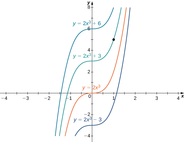 are displayed. The function satisfies the differential equation and the initial condition
Solving an Initial-Value Problem
Solve the initial-value problem

Solution
First we need to solve the differential equation. If  then
then

Next we need to look for a solution that satisfies the initial condition. The initial condition  means we need a constant such that
  Therefore,

The solution of the initial-value problem is 
Solve the initial value problem 
Solution

Hint
Find all antiderivatives of 
Initial-value problems arise in many applications. Next we consider a problem in which a driver applies the brakes in a car. We are interested in how long it takes for the car to stop. Recall that the velocity function is the derivative of a position function  and the acceleration is the derivative of the velocity function. In earlier examples in the text, we could calculate the velocity from the position and then compute the acceleration from the velocity. In the next example we work the other way around. Given an acceleration function, we calculate the velocity function. We then use the velocity function to determine the position function.
Decelerating Car
A car is traveling at the rate of 88 ft/sec  mph) when the brakes are applied. The car begins decelerating at a constant rate of 15 ft/sec2.
- How many seconds elapse before the car stops?
- How far does the car travel during that time?
Solution
- First we introduce variables for this problem. Let
 be the time (in seconds) after the brakes are first applied. Let be the acceleration of the car (in feet per seconds squared) at time
  Let be the velocity of the car (in feet per second) at time Let be the car’s position (in feet) beyond the point where the brakes are applied at time
The car is traveling at a rate of Therefore, the initial velocity is
  ft/sec. Since the car is decelerating, the acceleration is

The acceleration is the derivative of the velocity,

Therefore, we have an initial-value problem to solve:

Integrating, we find that

Since
 Thus, the velocity function is
To find how long it takes for the car to stop, we need to find the time
such that the velocity is zero. Solving  we obtain
  sec.
sec. - To find how far the car travels during this time, we need to find the position of the car after
 sec. We know the velocity is the derivative of the position
  Consider the initial position to be
  Therefore, we need to solve the initial-value problem

Integrating, we have

Since
 the constant is
  Therefore, the position function is
After
sec, the position is  ft.
ft.
Suppose the car is traveling at the rate of 44 ft/sec. How long does it take for the car to stop? How far will the car travel?
Show Answer

Hint

Key Concepts
- If is an antiderivative of then every antiderivative of is of the form for some constant
- Solving the initial-value problem

requires us first to find the set of antiderivatives of
and then to look for the particular antiderivative that also satisfies the initial condition.
For the following exercises, show that  are antiderivatives of
1. 
Solution

2. 
3. 
Solution

4. 
5. 
Solution

For the following exercises, find the antiderivative of the function.
6. 
7. 
Solution

8. 
9. 
Solution

For the following exercises, find the antiderivative of each function
10. 
11. 
Solution

12. 
13. 
Solution

14. 
15. 
Solution

16. 
17. 
Solution

18. 
19. 
Solution

20. 
21. 
Solution

22. 
23. 
Show Answer

24. 
25. 
Solution

For the following exercises, evaluate the integral.
26. 
27. 
Show Answer
28. 
29. 
Solution

30. 
31. ![\int (4\sqrt{x}+\sqrt[4]{x})dx](https://ecampusontario.pressbooks.pub/app/uploads/quicklatex/quicklatex.com-b28630a84f34f3cf7c8d498f6eae83ce_l3.png "Rendered by QuickLaTeX.com")
Solution

32. 
33. 
Solution

34. 
For the following exercises, solve the initial value problem.
35. 
Solution

36. 
37. 
Solution

38. 
39. 
Solution

For the following exercises, find two possible functions given the second- or third-order derivatives.
40. 
41. 
Solution
Answers may vary; one possible answer is 
42. 
43. 
Answers may vary; one possible answer is 
44. 
45. A car is being driven at a rate of 40 mph when the brakes are applied. The car decelerates at a constant rate of 10 ft/sec2. How long before the car stops?
Solution
5.867 sec
46. In the preceding problem, calculate how far the car travels in the time it takes to stop.
47. You are merging onto the freeway, accelerating at a constant rate of 12 ft/sec2. How long does it take you to reach merging speed at 60 mph?
Solution
7.333 sec
48. Based on the previous problem, how far does the car travel to reach merging speed?
49. A car company wants to ensure its newest model can stop in 8 sec when traveling at 75 mph. If we assume constant deceleration, find the value of deceleration that accomplishes this.
Solution
13.75 ft/sec2
50. A car company wants to ensure its newest model can stop in less than 450 ft when traveling at 60 mph. If we assume constant deceleration, find the value of deceleration that accomplishes this.
For the following exercises, find the antiderivative of the function, assuming 
51. [T] 
Solution

52. [T] 
53. [T] 
Show Answer

54. [T] 
55. [T] 
Solution

56. [T] 
For the following exercises, determine whether the statement is true or false. Either prove it is true or find a counterexample if it is false.
57. If is the antiderivative of  then
then  is the antiderivative of
Solution
True
58. If is the antiderivative of then  is the antiderivative of
59. If is the antiderivative of then  is the antiderivative of
Solution
False
60. If is the antiderivative of then  is the antiderivative of
Glossary
- antiderivative
- a function such that for all in the domain of is an antiderivative of
- indefinite integral
- the most general antiderivative of is the indefinite integral of
 we use the notation to denote the indefinite integral of
- initial value problem
- a problem that requires finding a function that satisfies the differential equation together with the initial condition

Hint
What function has a derivative of