3.3 Organizing Data
Using Microsoft Excel is one way we can organize and analyze descriptive data. The basic features of Excel are a row, column, and cell to organize data. The rows and columns in Excel form the software’s tabular format. Rows run horizontally, and Columns run vertically across the worksheet, with each row and column intersection point forming a Cell. While rows are denoted by numbers, columns are denoted by headers containing alphabets. A combination of Cells is a range.
Video: “Microsoft Excel. Working With Rows and Columns for Beginners” by Append Training is licensed under the Standard YouTube License [2:46] Transcript and closed captions available on YouTube.
Variables can be compared using the rows and columns. In Figure 3.3.1, the two variables are the patient’s age and height (HT):
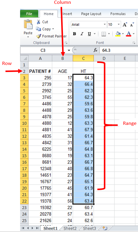
Image Description
The image shows an open Microsoft Excel spreadsheet with data and a “Sort” dialogue box overlay. The spreadsheet contains three columns labelled “PATIENT,” “AGE,” and “HT.” The first few rows of the data are visible with the following values:
| PATIENT | AGE | HT |
|---|---|---|
| 295 | 57 | 62.3 |
| 292 | 58 | 68.4 |
| 286 | 59 | 71.2 |
| 280 | 61 | 70.6 |
| 289 | 61 | 72.1 |
| 284 | 62 | 61.5 |
| 285 | 62 | 65.2 |
| 290 | 62 | 72.6 |
| 276 | 63 | 65.0 |
In the “Sort” dialogue box, there are options to add or delete levels for sorting. The current setting is:
- Column: AGE
- Sort On: Values
- Order: Smallest to Largest
There is a checkbox labelled “My data has headers” at the top of the dialogue box, and it is checked. Below this checkbox are buttons to manage the sort levels and to run or cancel the sort.
You can then sort and filter your data by column. For example, if I wanted to organize the data in the example table provided by age.
- Select data
- Within the HOME Ribbon (tab), select the Sort & Filter dropdown menu button (inverted triangle next to the word “Filter”) and select the “Custom Sort…” option.
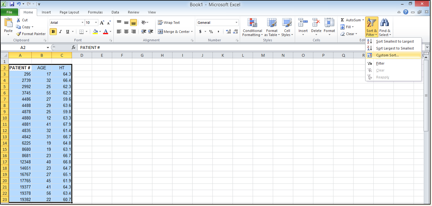
Image Description
This image depicts a screenshot of a Microsoft Excel 2010 spreadsheet. The spreadsheet interface includes the title bar at the top, which displays “Book1 – Microsoft Excel,” indicating it is an unsaved new workbook.
Below the title bar is the ribbon, an area that contains several tabs, including “File,” “Home,” “Insert,” “Page Layout,” “Formulas,” “Data,” “Review,” and “View.” The “Home” tab is currently selected and active, with a variety of formatting options displayed in the ribbon, such as “Clipboard,” “Font,” “Alignment,” “Number,” “Styles,” “Cells,” and “Editing.”
The worksheet grid is displayed below the ribbon. Columns are labelled with letters (A, B, C, D, etc.) along the top, and rows are labelled with numbers (1, 2, 3, etc.) down the left-hand side.
The range of cells from A1 to E20 is selected and highlighted in blue. The selected area appears to contain data, with the first column (A) showing a sequence of dates and the second column (B) corresponding values. The remaining columns seem to be empty.
On the far right side of the ribbon, a drop-down menu is visible under the “Sort & Filter” option, with the choices “Sort A to Z,” “Sort Z to A,” “Custom Sort,” and a separator with options below.
- The Sort box will appear, and under the Column heading, in the “Sort by:” category, select AGE. Under the Order heading, ensure “Smallest to Largest” has been selected. Click on OK
- Check to make sure the new dataset is correct.
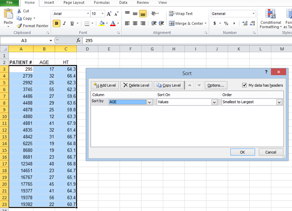
Image Description
The image shows an open Microsoft Excel spreadsheet with data and a “Sort” dialogue box overlay. The spreadsheet contains three columns labelled “PATIENT,” “AGE,” and “HT.” The first few rows of the data are visible with the following values:
| PATIENT | AGE | HT |
|---|---|---|
| 295 | 57 | 62.3 |
| 292 | 58 | 68.4 |
| 286 | 59 | 71.2 |
| 280 | 61 | 70.6 |
| 289 | 61 | 72.1 |
| 284 | 62 | 61.5 |
| 285 | 62 | 65.2 |
| 290 | 62 | 72.6 |
| 276 | 63 | 65.0 |
In the “Sort” dialogue box, there are options to add or delete levels for sorting. The current setting is:
- Column: AGE
- Sort On: Values
- Order: Smallest to Largest
There is a checkbox labelled “My data has headers” at the top of the dialogue box, and it is checked. Below this checkbox are buttons to manage the sort levels and to run or cancel the sort.
Video: “Excel: Sorting Data” by LearnFree is licensed under the Standard YouTube License [4:30] Transcript and closed captions available on YouTube.
 Applying Your Knowledge
Using the following image:
- Identify the row, column, cell and range.
- What is the value in cell C18?
- What is the range of cells selected?
- What is the independent variable?
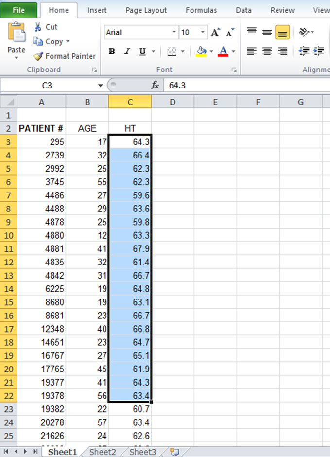
Image Description
The image is a screenshot of a Microsoft Excel spreadsheet. The spreadsheet displays three columns labelled “PATIENT #,” “AGE,” and “HT,” with data entries in each column. Here is the detailed description of the data:
| PATIENT # | AGE | HT |
|---|---|---|
| 295 | 17 | 64.3 |
| 2739 | 32 | 66.4 |
| 2992 | 25 | 62.3 |
| 3745 | 55 | 62.3 |
| 4486 | 27 | 59.6 |
| 4488 | 29 | 63.6 |
| 4878 | 25 | 59.8 |
| 4880 | 12 | 63.3 |
| 4881 | 41 | 67.9 |
| 4835 | 32 | 61.4 |
| 4842 | 31 | 66.7 |
| 6225 | 59 | 64.8 |
| 8680 | 19 | 63.3 |
| 8681 | 23 | 66.7 |
| 12348 | 40 | 66.8 |
| 14651 | 23 | 64.7 |
| 16767 | 27 | 65.1 |
| 17765 | 45 | 61.9 |
| 19377 | 41 | 64.3 |
| 19378 | 56 | 63.4 |
| 19382 | 22 | 60.7 |
| 20278 | 57 | 63.4 |
| 21626 | 24 | 62.6 |
The spreadsheet interface includes the following tabs in the toolbar: “File,” “Home,” “Insert,” “Page Layout,” “Formulas,” “Data,” “Review,” and “View.” Various formatting options, such as font type, size, alignment, and styles, are present above the data. The “HT” column is highlighted in light blue.
Below the data area are sheet names “Sheet1,” “Sheet2,” and “Sheet3,” with “Sheet1” currently selected.
Microsoft Excel screenshots used with permission from Microsoft.
