3.4 Basic functions in Excel
Often, when collecting data, we will need to use formulas to determine things like count, averages, etc. You can use a cell in Excel to create a formula.
Video: “Excel: Intro to Formulas” by LearnFree is licensed under the Standard YouTube License [3:39] Transcript and closed captions available on YouTube.
In Excel, a function is a predefined formula that performs a specific calculation by using values a user inputs. You will see in the video there are many functions that can be used in place of formulas when using Excel. The most common functions we will use are found in Excel by clicking the Formulas ribbon and AutoSum.
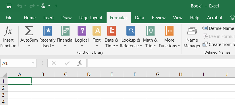
Image Description
The image is a screenshot of a Microsoft Excel interface.
At the topmost section, there is a green title bar displaying “Book1 – Excel” on the right side. Below that is a ribbon menu with the following tabs from left to right: File, Home, Insert, Draw, Page Layout, Formulas (selected), Data, Review, View, Help, and Acrobat. The Tell me what you want to do… search bar is next to these tabs on the right.
Underneath the ribbon menu, there’s a toolbar specific to the “Formulas” tab, divided into several groups:
- Function Library including icons for Insert Function, AutoSum, Recently Used, Financial, Logical, Text, Date & Time, Lookup & Reference, Math & Trig, More Functions
- Defined Names, including icons for Define Name, Use in Formula, Create from Selection
- Formula Auditing, including icons for Name Manager
Below this toolbar, there’s a standard Excel grid with columns labelled from A to I and rows labelled from 1 to 4.
A single cell, A1, is highlighted, indicating it is currently selected.
Here, you will find quick functions like Sum and Average.
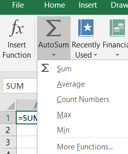
Image Description
The image is a screenshot of a section of the Microsoft Excel interface. The top menu bar displays the options “File,” “Home,” “Insert,” and “Draw.” Below this menu bar, there is a toolbar with various buttons and icons commonly used in Excel.
On the left side of the toolbar, there is an “fx” icon with the text “Insert Function” next to it. To the right, there is an “AutoSum” button denoted by a summation symbol (Σ). Next to the “AutoSum” button, there are two more buttons labelled “Recently Used” and “Financial.”
When the AutoSum button is clicked, a dropdown menu appears. This dropdown menu contains the following options:
- Sum
- Average
- Count Numbers
- Max
- Min
- More Functions…
Below the toolbar, a small portion of a worksheet is visible. The formula “=SUM(” is displayed in a highlighted cell, indicating that the user is currently entering a SUM function.
You can also click Insert Function. If you are not sure, you can describe what you want to do, and Excel will recommend the function that may perform the formula you require.
The following video shows the basic function skills you may use.
Video: “Excel: Functions” by LearnFree is licensed under the Standard YouTube License [5:15] Transcript and closed captions available on YouTube.
 Applying Your Knowledge
- Open Excel.
- Create a worksheet and enter the data as shown in the image.
- Using functions in your worksheet calculate the average and median age.
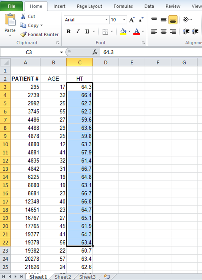
Image Description
This image shows an Excel spreadsheet with the following details:
– The title at the top left reads “File.”
– The horizontal menu options include Home, Insert, Page Layout, Formulas, Data, Review, and View. The “Home” tab is currently selected.
– Below the menu options, there are various buttons and tools, such as Clipboard, Font settings, Alignment, and Number formatting.
– The sheet has three columns with headers: “PATIENT #”, “AGE”, and “HT.”
The table data begins from row 2 and continues downwards. Here is a description of the table:
| PATIENT # | AGE | HT |
|---|---|---|
| 295 | 17 | 64.3 |
| 2726 | 37 | 69.2 |
| 3078 | 55 | 66.4 |
| 3176 | 43 | 62.6 |
| 4439 | 52 | 66.3 |
| 4575 | 41 | 63.4 |
| 4818 | 40 | 68.7 |
| 4831 | 57 | 61.8 |
| 4839 | 47 | 67.1 |
| 4881 | 25 | 64.4 |
| 4884 | 32 | 63.3 |
| 5065 | 23 | 64.8 |
| 5104 | 33 | 62.4 |
| 10577 | 47 | 68.1 |
| 14005 | 46 | 63.9 |
| 15835 | 30 | 65.5 |
| 16764 | 27 | 67.3 |
| 16677 | 29 | 64.9 |
| 17864 | 39 | 61.8 |
| 23472 | 23 | 62.4 |
| 23482 | 55 | 62.7 |
The HT column from C2 to C23 is highlighted in a light blue colour.
Microsoft Excel screenshots used with permission from Microsoft.
