8.2. Solved Examples: Tension and Compression
Tension questions with multiple cables (strings, ropes) involved. Solved example
The system in the picture is used to suspend a 10 kg object. Find the tensions in the ropes.
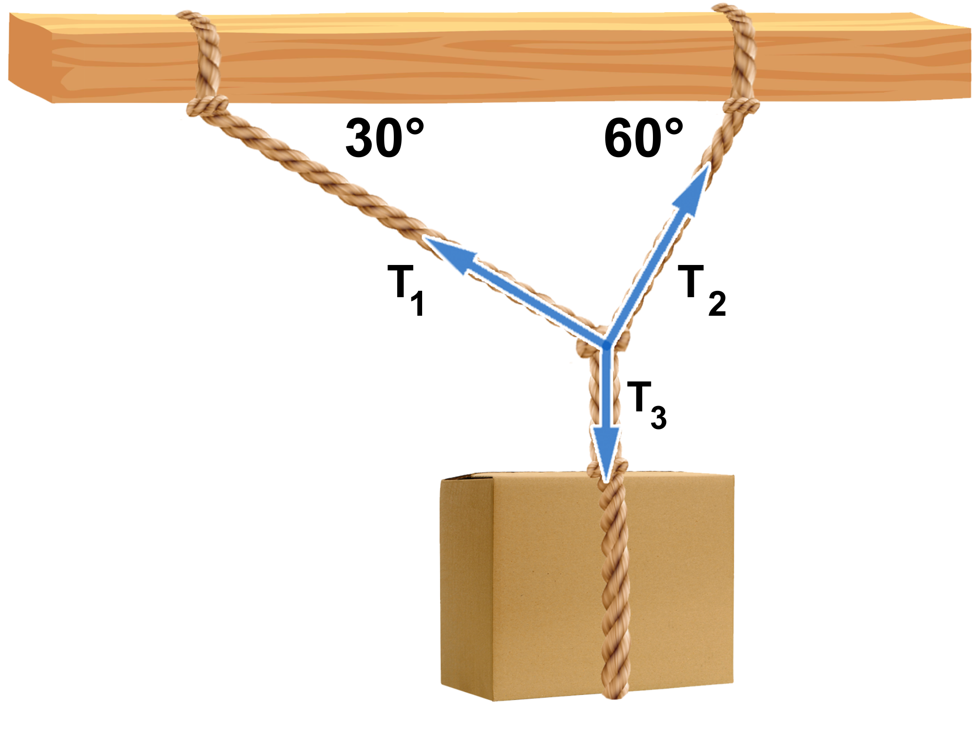
We once again imagine that we cut the ropes and replace their effect by the respective forces of tension.
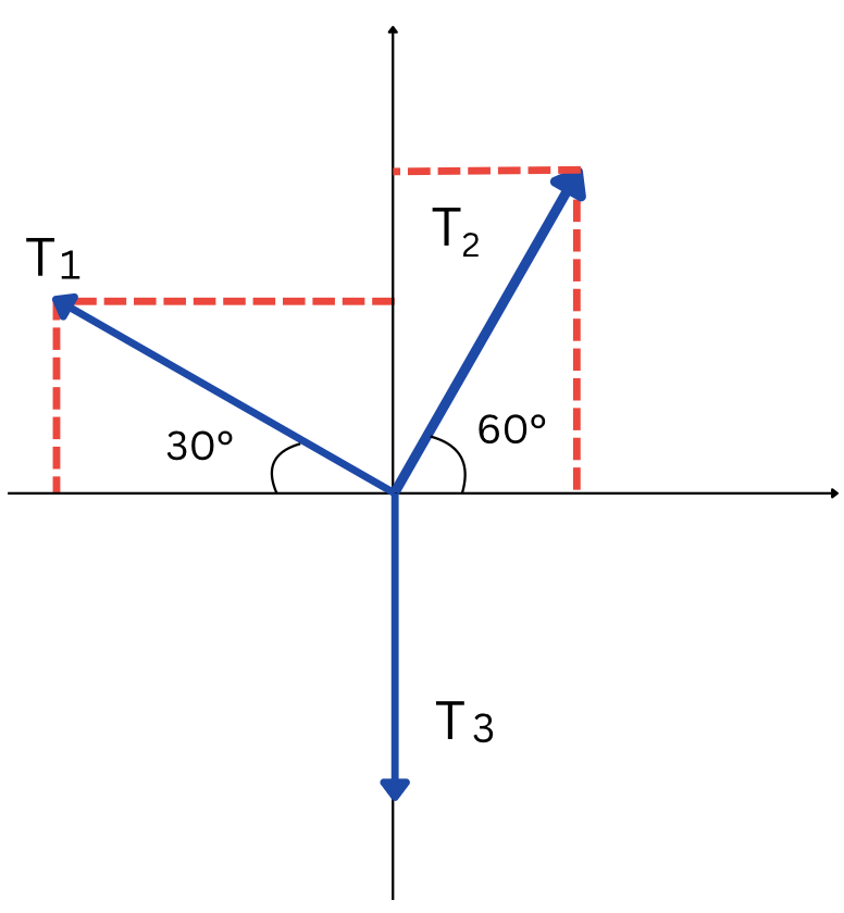
The FBD for the system is represented in figure 8.4 b). The tension in cable 3, [latex]T_3[/latex], will be equal to the weight of the hanging load:
[latex]T_3 = F_g = m \hspace{.2cm} \text × \hspace{.2cm}g = 10 \hspace{.2cm} \text × \hspace{.2cm}9.8 = 98 \hspace{.2cm} \text N[/latex]
To solve the system and find the other two tensions ([latex]T_1[/latex] and [latex]T_2[/latex]), we can organize the calculations in a table (presented below). The table is used to resolve all forces on the x and y axes, so that we can express the net force on the x axis, respectively on the y axis. Since the system is in equilibrium on these axes, both net forces will be zero.
| Vector | X-Components | Y-Components |
|---|---|---|
| [latex]T_1[/latex] | [latex]-T_1 \hspace {.2cm} \text {cos} \hspace {.2cm} 30^ \circ[/latex] | [latex]T_1 \hspace {.2cm} \text {sin} \hspace {.2cm} 30^ \circ[/latex] |
| [latex]T_2[/latex] | [latex]T_2 \hspace {.2cm} \text {cos} \hspace {.2cm} 60^ \circ[/latex] | [latex]T_2 \hspace {.2cm} \text {sin} \hspace {.2cm} 60^ \circ[/latex] |
| [latex]T_3[/latex] | [latex]0[/latex] | [latex]- \hspace {.2cm} 98[/latex] |
| Total | [latex]-T_1 \cos 30^\circ + T_2 \cos 60^\circ[/latex] | [latex]T_1 \sin 30^\circ + T_2 \sin 60^\circ - 98[/latex] |
Conditions for Equilibrium
Since the system is in equilibrium on both axes:
[latex]F_{\text{net},x} = 0; \quad -T_1 \cos 30^\circ + T_2 \cos 60^\circ = 0 \quad (1)[/latex]
[latex]F_{\text{net},y} = 0; \quad T_1 \sin 30^\circ + T_2 \sin 60^\circ - 98 = 0 \quad (2)[/latex]
Solving the system of two equations with two variables results in:
[latex]T_1 = 49 \hspace{.2cm} \text N,\hspace{.2cm} T_2 = 85 \hspace{.2cm} \text N[/latex]
Tension and compression question. Example solved
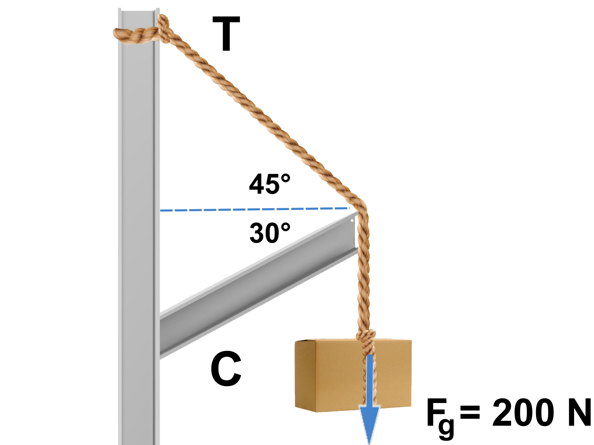
The metallic bar in the figure is being pressed, thus developing a compression in the bar. The bar reacts with a force that we call the equilibrant force, denoted by [latex]E[/latex] (it is the force that produces the equilibrium in the system).The equilibrant force is equal in magnitude and opposite in direction with compression, denoted by [latex]C[/latex].
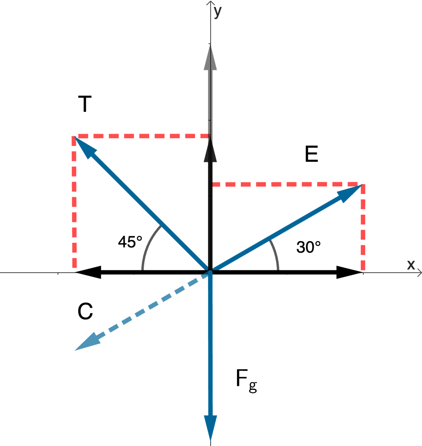
Similar to the previous question, we can organize the calculations in a table (presented below). The table is used to resolve all forces on the x and y axes, so that we can express the net force on the x axis, respectively on the y axis.
Since the system is in equilibrium on these axes, both net forces will be zero.
| Vector | X-Components | Y-Components |
|---|---|---|
| [latex]T[/latex] | [latex]- T \hspace{.2cm} \text {cos} \hspace{.2cm}45°[/latex] | [latex]T \hspace{.2cm} \text {sin} \hspace{.2cm}45°[/latex] |
| [latex]E[/latex] | [latex]E \hspace{.2cm} \text {cos} \hspace{.2cm}30°[/latex] | [latex]E \sin 30^\circ[/latex] |
| [latex]F_g[/latex] | [latex]0[/latex] | [latex]- \hspace{.2cm}200[/latex] |
| Total | [latex]-T \cos 45^\circ + E \cos 30^\circ[/latex] | [latex]T \sin 45^\circ + E \sin 30^\circ - 200[/latex] |
Conditions for equilibrium:
[latex]F_{\text{net},x} = 0; \quad -T \cos 45^\circ + E \cos 30^\circ = 0 \quad (1)[/latex]
[latex]F_{\text{net},y} = 0; \quad T \sin 45^\circ + E \sin 30^\circ - 200 = 0 \quad (2)[/latex]
Solving the system of two equations with two variables results in:
[latex]E = C =\hspace{.2cm} 146.4 \hspace{.2cm} \text N[/latex]
[latex]T = \hspace{.2cm} 179.4 \hspace{.2cm} \text N[/latex]
Image Attributions
- Figures 8.4 and 8.5 adapted from:
- Rope by pikisuperstar courtesy of Freepik
- Wooden beam by pch.vector courtesy of Freepik
- Cardboard box by kstudio courtesy of Freepik
- Metal beam by upkylak courtesy of Freepik
- Geometric figure adapted from Geogebra and licensed under CC-BY-NC-SA 3.0.
