Introduction

Daniel FitzGreen

Optical Tweezers

Introduction

The concept of optical tweezers won the Nobel prize in physics in 2018. In this technique, laser light is focused on a specimen and the gradient of the laser power holds the sample in place. Optical Tweezers have been used to capture live bacteria [1] and to study the intermolecular forces of DNA [2].

2.1 The Physics of Optical Tweezers

The physics that describes optical tweezers is separated into two regimes that depend on the relative magnitude of the laser wavelength ( $\lambda$ ) and the radius of the trapped particle ( $R$ ). Please know that there are equations that describe the forces in each regime, but since you don’t need them for the analysis, they have been omitted. It is incredibly important that you have a conceptual understanding of the physics, and appreciate the assumption of the harmonic potential and how that makes the analysis possible.

2.1.1 The Mie Regime ( $R>>\lambda$ )

In this regime, the laser light is treated as a collection of photons with nearly identical momenta ( $p=h\lambda$ ). If those photons were to refract at the boundary between the sample particle and its surrounding medium, then the photon would impart some small amount of momentum to the sample particle. The total net momentum from all of the photons in the laser beam will generate a net radiation pressure on the sample. Consider photons from a laser beam and a spherical sample particle as in Figure 1. The photons refract at each boundary and exit the sphere with a new trajectory. The magnitude of the photon’s momentum remained constant, but its direction changed. The momentum of the sphere must also have changed for the total momentum to remain conserved. A photon entering the sphere on the left will exit to the right, thereby pushing the sphere more to the left and vice versa. The center of the Gaussian is to the left of the center of the sphere, which pushes the sphere towards the center of the Gaussian photon distribution. With enough laser power, the force towards the center of the laser beam is sufficient and the sphere is trapped in the xy plane.

You may have noticed from Figure 1 that the net force from the Gaussian beam (called $F_g$ ) will have a component that pushes the sphere downstream. Not only that, but some photons scatter or reflect off of imperfections in the sphere, which imparts much more momentum in the forward dimension than a photon that travels through (this scattering/reflection ( $F_s$ ) is actually the dominant effect). Trapping in the z-axis is achieved by focusing the laser beam with a lens that has a very large numerical aperture, as in Figure 2.

Figure 1: Gaussian laser beam profile refracting through a sphere. The refraction results in a net force towards the center of the beam.

Figure 2: Ray diagram depicting the forces that trap the sphere in the z-axis

When the center of the sphere is upstream from the focal point of the laser, the net force pushes the sphere downstream, as it did with the collimated laser. When the sphere is pushed downstream of the focal point of the beam, $F_g$ changes direction and pushes the sphere back upstream. The result is that the sphere becomes trapped just a bit downstream from the focal point of the laser.

2.1.2 The Rayleigh Regime ( $R<<\lambda$ )

In the Rayleigh regime, the sphere is much smaller than the wavelength of light, and we can no longer treat the laser as a collection of photons. Instead, the physics is described by waves of electromagnetic radiation that displace the electrons from their nuclei, then the bead is treated as a dipole. The dipole oscillates as the electromagnetic wave passes through it and radiates secondary waves which mix with the incident EM wave from the laser. The change in momentum of the incident and outgoing wave is imparted to the sphere, much like in the Mie regime with individual photons. Though the physics of this situation is different than in the Mie regime, the result is the same: The sphere is trapped a bit downstream from the focal point of the laser.

2.1.3 In Between ( $R \approx \lambda$ )

We can trap samples in the Mie and Rayleigh regimes, so it shouldn’t be too surprising to learn that the sample is trapped when ( $R\approx\lambda$ ). Understanding the physics in this in-between regime requires complex mathematical models that don’t have analytic solutions. But when these models are solved, the result is the same: The sphere is trapped just downstream of the focal point of the lens. What is also true about all of these regimes is that the stiffness of the trap is dependent on the power of the laser.

2.2 Trap Stiffness

As you read the previous section, you might have realized that the restoring force on the sphere is proportional its distance from the laser center – much like a spring. You may remember the term ‘harmonic potential’, described by the equation

(1) $\begin{equation*} V(x) = \cfrac{1}{2}kx^2, \end{equation*}$

where $k$ is the spring constant and x is the distance from equilibrium. The restoring force is then $F=kx$ . It is assumed that the sphere is close to the center of the laser and so it is relatively close to the bottom of the potential well in which it is trapped, then the assumption of the harmonic potential is a good one. The analogy to the spring constant is the trap stiffness (also $k$ ), which can be measured in multiple ways with this apparatus.

2.2.1 Equipartition

A bead that finds its way within the edges of the trap will move towards the trap center, quickly losing energy through drag in the surrounding fluid and settling to the bottom of the trap. The bead is in thermal equilibrium with the surrounding medium, so the average kinetic energy of the bead will follow the Maxwell-Boltzmann distribution. The bead is then presumed to undergo Brownian motion as a result of random interactions with the molecules of the surrounding medium. Inside the trap, the beads are still affected by the same forces, but will be held roughly centered by the trap potential. If the trap potential for small displacements is modeled as a harmonic potential, the equipartition theorem can be applied to equate the thermal energy for each degree of freedom, shown here for the x direction:

(2) $\begin{equation*} \cfrac{1}{2}k_BT = \cfrac{1}{2}k_x \langle (x-\overline{x})^2\rangle.\end{equation*}$

Therefore, if we know the temperature and take many measurements of the position of the bead, then the trap stiffness can be determined. Note that one does not need to accurately know the size of the bead, what it’s made of, or anything about the surrounding medium other than its temperature. Pretty powerful little theorem, there!

In this experiment, the quadrant pole detector (QPD) (explained in Section 3.5.1) is used to make many measurements of the bead position very rapidly, then the output of the QPD is calibrated using a stuck bead of known size.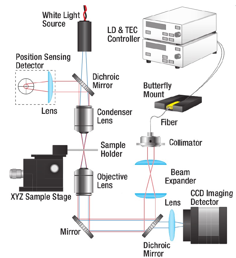

Figure 3: Schematic of optical tweezers apparatus. Note the paths of the laser (red) and white light (blue).

2.2.2 Stoke’s Drag

The Stoke’s Drag method relies on applying a known force (namely, the drag force on the bead) to probe the stiffness of the trap. The drag force is induced by moving the trap at a known (or measured) velocity as the position of the bead is continuously measured using the QPD.

Stoke’s law states that the force on a small sphere moving through a viscous fluid is given by

(3) $\begin{equation*} F_d = 6\pi\mu R\nu,\end{equation*}$

where $F_d$ is the drag force, $R$ is the radius of the sphere, $\mu$ is the dynamic viscosity of the medium and $\nu$ is the velocity of the sphere. Since the trap is modelled as a harmonic potential, the drag force should be proportional to the distance from the trap axis ( $F_d =kx$ ). The trap stiffness can then be determined by taking position measurements with various velocities and knowing the values of the constants in Equation (3).

Introduction