Introduction

Daniel FitzGreen

Li(p,n)

Introduction

Bombarding lithium with protons is a well-established method for producing a near mono-energetic beam of neutrons. These neutrons are often used in cancer treatment [2] and to perform neutron activation analysis of human bones [1].

2.1 Li(p,n)

Nuclear physicists take advantage of the following reaction to generate a beam of neutrons:

(1) $\begin{equation*} \ce{^7Li(p,n)}\ce{^7Be} \end{equation*}$

It’s not the clearest notation, but basically, the incoming proton transfers its energy to a neutron in the lithium nucleus. The result is a beryllium isotope with 4 protons and 3 neutrons ( $\ce{^7Be}$ ) and an excess neutron. This transfer of energy only works at specific values of the proton energy (you can thank quantum mechanics for that). Reactions that occur at specific energies like this are generally referred to as resonances. There are actually two resonances here, depending on the proton energy. A spectrum with these resonances is shown in Figure 1. The first produces a neutron and a $\ce{^7Be}$ in its ground state. This resonance at 1.881 MeV is called a threshold resonance since there is no neutron production at lower energies. This resonance is VERY asymmetric and VERY broad. The second resonance generates a slightly-faster neutron and the beryllium in an excited state ( $\ce{^7Be}^*$ ). This is a more usually-shaped resonance at about 2.3 MeV.

The y-axis of the plot in Figure 1 is the cross section of the interaction, which is in units of area $^{-2}$ , much like a physical cross section would have. The unit of choice in these types of scattering/resonance experiments is the barn, which is $10^{-28}$ m $^2$ , a.k.a. 100 fm $^2$ . The cross section is a measure of the probability of the given interaction – in this case the interaction that generates neutron from the lithium and incoming proton. The cross section for these interactions (and generally, these types of interactions) is described by the Breit Wigner formula.

2.2 Breit Wigner Distribution

The Breit Wigner distribution describes resonances in nuclear scattering experiments and in gamma spectroscopy. You may know this function as the Cauchy or Lorentz distribution. Also note that this is NOT the relativistic Breit Wigner distribution.

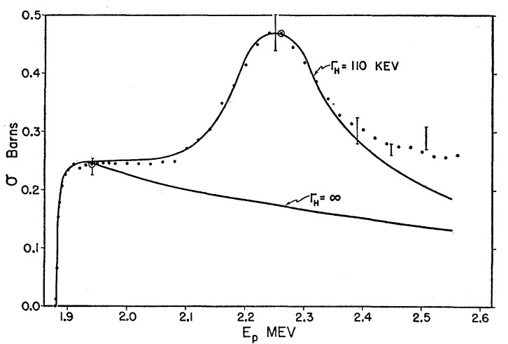
(2) $\begin{equation*} \sigma = \cfrac{1}{\pi} \cfrac{\Gamma}{(E-E_0)^2+(\Gamma/2)^2},\end{equation*}$

Figure 1: Cross section for neutron production as a function of proton energy. Note the two resonances that generate protons: the threshold at 1.881 MeV (lower curve) and the resonance at about 2.3 MeV (upper curve). Figure from Reference [4].

where $\sigma$ is the cross section of the interaction, $\Gamma$ is the width of the interaction (i.e. the probability of interaction within a specific time), $E$ is the energy of the incoming particle, and $E_0$ is the energy of the resonance. Note that this distribution is normalized. When you are fitting data, your fit functions do not have to be normalized; your amplitude can be arbitrary. The Li(p,n) resonance at 2.3 MeV is a good example of this distribution.

The Breit-Wigner equation for Li(p,n) is slightly complicated by the existence of an intermediate, compound state. The reaction actually proceeds by the proton and lithium forming a compound state, then that compound state decays, with a probability of resulting in a neutron. Therefore, the numerator has two separate width terms: One for the creation of the compound state, and one for the decay:

(3) $\begin{equation*} \sigma_{(p,n)}(E^{CM}_p)=\pi \lambda^2_p g(J)\cfrac{\Gamma_p\Gamma_n}{(E^{CM}_p-E_r)^2+\Gamma^2/4},\end{equation*}$

where $\Gamma_p$ and $\Gamma_n$ are the proton and neutron widths. The total width $\Gamma = \Gamma_p + \Gamma_n$ . The proton energy in the center of mass frame is $E^{CM}_p$ and $E_r$ is the energy of the resonance. The deBroglie wavelength of the proton ( $\lambda_p$ ) is inversely proportional to the proton energy $(\lambda_p \propto 1/E_p)$ . The factor $g(J)$ takes the particles’ spin into account: $g(J) = (2J +1)/[(2S+1)(2I+1)]$ where $S$ is the proton spin and $I$ is the total spin of the target nucleus. Assuming $\ell$ = 0, then $I = 3/2$ for the Li nucleus, then $g(J)= 5/8$ . Note that the only difference between this equation and Equation (2) is the extra width term and a non-arbitrary amplitude term. The energy difference in the denominator is very small near the threshold resonance, and can be neglected. The above equation can be rearranged to be in terms of the proton and neutron widths individually:

(4) $\begin{equation*} 4\pi \lambda^2_pg(J)\cfrac{\Gamma_n\Gamma_p}{(1+\Gamma_n/\Gamma_p)^2}. \end{equation*}$

Working with the width of these interactions is awkward since we don’t actually control them. We take advantage of the fact that $\Gamma_n/\Gamma_p \propto \sqrt{1-E_{th}/E_p}.$ If one calculated all of these constants, as they did in reference [3], one would find the differential cross section to be

(5) $\begin{equation*} \cfrac{\dd\theta}{\dd\Omega^{CM}}(E_p) = \cfrac{169.72\text{MeV mb/sr}}{E_p} \cfrac{x}{(1+x)^2},\end{equation*}$

where $x=C\sqrt{1-E_{th}/E_p}$ , where $C$ is some dimensionless constant that is determined through fitting the data. Therefore, the two unknown parameters are $C$ and $E_{th}$ . Note that this function is undefined where $E_p < E_{th}$ , which makes the least-squares fir VERY dependent on the initial guess values of the parameters. Also note that the differential cross section is just the cross section per unit of solid angle. Since various detector setups will cover various solid angles, results are typically normalized to the solid angle

2.3 Tandem Accelerator

Early particle accelerators often used high voltage from a Van der Graff style generator to accelerate ions like protons (which is also an $\ce{H^+}$ ion). A later iteration of electrostatic accelerator, called a tandem accelerator or Tandetron, changes the charge on the accelerated ion in order to use the high voltage twice.

The Tandetron, shown in Figure 2, starts with $\ce{H^-}$ ions. The negative ions are accelerated by the high voltage towards a thin carbon foil or gas mixture where the electrons are stripped without slowing down the ion. The newly-made $\ce{H^+}$ is now accelerated from the high voltage to the output of the accelerator. With this setup, the output proton beam has been accelerated twice by a single high voltage. Magnetic and electrostatic fields focus and steer the proton beam to the target sample.

Figure 2: Schematic diagram showing the working principle of a tandem accelerator. Negative ion are accelerated by the increasing voltage towards the electron stripper and the resulting positive ions are accelerated by the decreasing voltage, thereby using just one high-voltage supply. The positive ions (protons) are electrostatically and magnetically steered towards the lithium target to generate neutrons.

2.4 BF₃ Detector

The $\ce{BF_3}$ detector is so names because it uses boron trifluoride gas that has been enriched to contain an unnatural amount of $\ce{^{10}B}$ . Neutrons react with the $\ce{^{10}B}$ to produce alpha particles (basically a helium nucleus). These alpha particles ionize the gas in the detector in the presence of a large electric field that accelerates the ionized electrons toward a central anode, thereby generating an electric pulse. There are a few important limitations that one needs to understand before trusting $\ce{BF_3}$ detector counts:

The detector preferentially detects slow, or moderated, neutrons. Good moderating materials include graphite, water, or paraffin wax.
The detection efficiency decreases as $1/v$ , so neutrons travelling twice as fast have half the chance to be detected.
The $\ce{BF_3}$ detector does not only detect neutrons. Low-energy gamma rays, specifically X-rays, are efficiently detected and must not be confused for neutrons.
$\ce{BF_3}$ detectors are proportional, meaning that you can measure the energy spectrum of the incoming neutrons (much like in gamma spectroscopy)

The output of the detector is passed various amplifiers and pulse shapers before it is counted. These values need to be set and remain consistent for the entire experiment. The detector output is counted using a multi-channel analyzer (MCA) and the computer software displays a histogram of the counts as a function of energy.

Introduction

2.1 Li(p,n)

2.2 Breit Wigner Distribution

2.3 Tandem Accelerator

2.4 BF₃ Detector

License

Share This Book

2.1 Li(p,n)

2.2 Breit Wigner Distribution

2.3 Tandem Accelerator

2.4 BF3 Detector

License

Share This Book

2.4 BF₃ Detector