Introduction

Daniel FitzGreen

Torsional Oscillator

Introduction

The TeachSpin manual (which can be found here) has a lot of info you will need, particularly Chapter 4, which forms the basis of the experiments you will do in your lab session.

Damped Harmonic Oscillation

Hopefully you remember some details about harmonic oscillators from your 2nd and 3rd year physics courses. The defining concept in harmonic oscillators is that they are driven by a restoring force

(1) $\begin{equation*} F=m\cfrac{d^2x}{dt^2} = -kx, \end{equation*}$

where $k$ is some positive constant and $x$ is some kind of displacement from equilibrium. The most common example you’ve seen is likely a mass on a spring, where $k$ is the spring constant and $x$ is how far the spring is stretched, but many systems exhibit harmonic oscillation, such as inductor-capacitor (LC) circuits, changes in predator-prey numbers, and in the muscle tension of a beating heart.

In this torsional oscillator, the solution to Equation (1) is $x(t)=\theta(t) = A*sin(\sqrt{\kappa/I})*t)$ , where constant the $k$ from Equation 1 is $\sqrt{\kappa/I}$ , where $\kappa$ is the torsion constant of wire (similar to spring constant) and $I$ is the rotational inertia, similar to mass.

Of course, nothing lasts forever in this universe. Your harmonic oscillators will always be subject to some form of energy loss, usually in the form of friction. The friction force is often (but not always) proportional to the velocity of the object that is oscillating, which adds a new force to Equation 1:

(2) $\begin{equation*} F=m\cfrac{d^2x}{dt^2} = -kx-c\cfrac{dx}{dt} \end{equation*}$

where $c$ is some damping coefficient. The solution to this equation in the damped torsional oscillator is

(3) $\begin{equation*} \theta(t) = A*\exp[-\gamma \omega_0 t]*\cos[\omega_0 (\sqrt{1-\gamma^2})t], \end{equation*}$

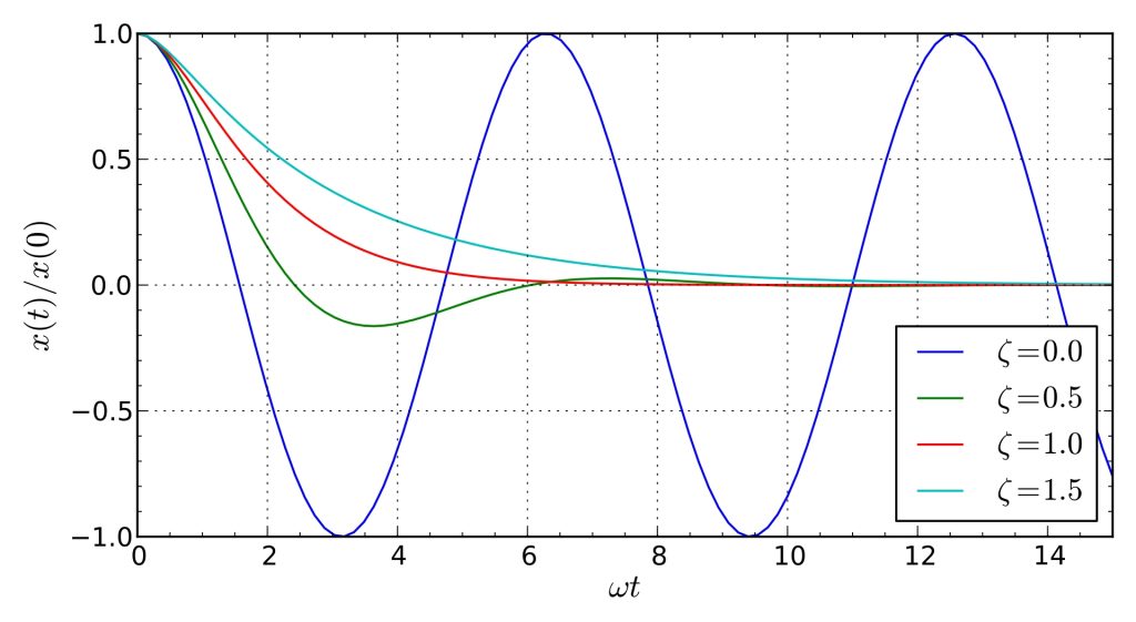
where $\omega_0$ is the angular frequency of the undamped motion and $\gamma$ is a dimensionless parameter that quantifies the amount of damping. You have probably seen a function that looks something like the green curve in Figure 1, where the amplitude of the oscillations decreases exponentially while the period stays the same.

A more general form of Equation 3 (used or fitting data, for example) is

(4) $\begin{equation*} \theta(t) = A*\exp[-B t]*\cos[Ct-D]+E, \end{equation*}$

where $A$ , $D$ , and $E$ are set by the initial conditions (hopefully it’s clear to you how those values change the function). B and C should be independent of initial conditions, and also follow the rule

(5) $\begin{equation*} B^2+C^2=\omega_0^2. \end{equation*}$

Even though B and C each depend on both $\gamma$ and $\omega_0$ , one can use the fit values to determine $\omega_0$ and $\gamma$ .

The “quality” of an oscillator is defined as $Q=1/(2\gamma)$ . A large $Q$ value indicates the system has very little damping, which is typically what oscillators are going for. The $Q$ value of an oscillator is used to define three regions of damped harmonic oscillation.

Underdamped

When $Q$ is greater than 0.5, the system is said to be damped, or underdamped. Motion that looks anything like the green curve in Figure 1 is underdamped.

Critically Damped

When $Q$ is exactly equal to 0.5, the system is said to be critically damped. When $Q=0.5$ , then $\gamma=1$ , and the sinusoidal behaviour in Equation 3 becomes a constant value of unity. The oscillator smoothly, and exponentially, approaches the equilibrium. A good example of a desired critically damped system would be an RL circuit used as filter. Ideally, the filter would remove as much unwanted noise as possible without continued oscillation, sometimes called ‘ringing’. An example of this “oscillation” is the red curve in Figure 1.

Overdamped

An overdamped system has a $Q$ value of (you guessed it!) less than 0.5. In this case, the oscillatory motion continues, though at a different frequency than in the undamped case. The light blue curve in Figure 1 is an example of overdamped oscillation.

Different Sources of Friction

The discussion above considered only damping that was linear with the speed of the oscillator (i.e. $v^1$ ), as shown in Figure 2b. Other sources of friction can be studied, though are much harder to model with potentially no analytic solution.

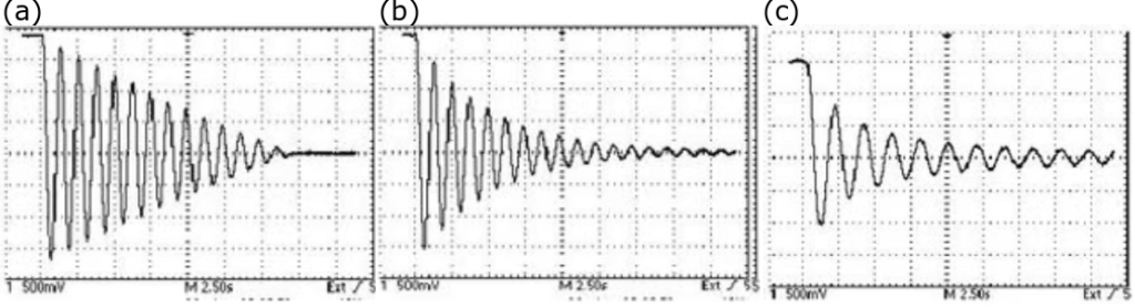examples of damping — Figure 2: Examples of (a) $v^1$ damping, (b) $v^0$ damping, and (c) $v^2$ damping.

Constant Friction ( $v^0$ )

Friction does not always necessarily depend on linearly on velocity, though. For example, a constant friction will linearly decrease the amplitude of oscillation, eventually to zero once the friction force is larger than the restoring force. Instead of the exponential decay of the amplitude as in Figure 2b, the amplitude decreases linearly, as in Figure 2a.

This type of damping can be achieved with static friction, like having a mass on a horizontal spring and not taking care to minimize friction between the mass and the surface it moves on. Or in the case of the torsional oscillator, by tying a string to rub against the rotor as it turns.

Fluid Friction ( $v^2$ )

Fluid friction depends on the square of the speed of the oscillator and becomes very difficult to model, which is kind of the hallmark of fluid dynamics. The fluids dynamics that describe how the fluid around the oscillator moves and drags is only relevant at relatively large velocity, so this source of friction can become negligible at very small amplitude, as in Figure 1c. The oscillations become anisochronous – the period is not constant. This motion is (double surprise!) difficult to model.

One can do a simple analysis where the data is fit with TWO exponential terms in the fit function – one that captures the rapid damping due to fluid friction AND the underdamping that becomes significant once the fluid friction is not. The changing period is not easily fit, but one will likely see evidence of this feature in the residuals of the fit.

Introduction

Damped Harmonic Oscillation

Underdamped

Critically Damped

Overdamped

Different Sources of Friction

Constant Friction ( $v^0$ )

Fluid Friction ( $v^2$ )

License

Share This Book

Damped Harmonic Oscillation

Underdamped

Critically Damped

Overdamped

Different Sources of Friction

Constant Friction ()

Fluid Friction ()

License

Share This Book

Constant Friction ( $v^0$ )

Fluid Friction ( $v^2$ )