Introduction

Daniel FitzGreen

Gravitational Lensing

Introduction

Though gravitational lensing is usually associated, and correctly described by, Einstein’s theory of general relativity, the phenomena is predicted by classic Newtonian physics. The amount of deflection is determined by integrating along the path of the photon moving by a point mass $M$ , as in Figure 1. The Newtonian deflection angle for the photon was found to be

(1) $\begin{equation*} \alpha = \cfrac{2GM}{c^2\xi},\end{equation*}$

Figure 1: A simple representation of gravitational deflection.

where $G$ is the gravitational constant, $c$ is the speed of light, and $\zeta$ is the ’impact parameter’ or distance of closest approach. In general relativity, 3D space is distorted by the gravitational field of massive bodies. A good analogy is a plastic film stretched across a hoop. Masses distort 3D space the way pushing down on the film with your finger distorts the film. In fact, this same analogy applies to electrostatics, and is the hallmark of a field that can be described by the Poisson equation (if this is the first time you are hearing about Poisson’s equation, please google/wiki it. It’s super powerful, and is a generalization of Laplace’s equation, which comes up a lot, too). Due to this distortion of space, one must account for gravitational effects on the spatial AND temporal components of the photons path, resulting in twice the deflection angle:

(2) $\begin{equation*} \alpha = \cfrac{2GM}{c^2\xi},\end{equation*}$

The first experimental verification of gravitational lensing came in 1919 during a total solar eclipse. Astronomers observed stars as their light passed by the Sun, and measured the difference between their known position and apparent positions. The deflection was measured to be 1.61 $\pm$ 0.40 arcseconds. Compare this measurement with the result of Equation (2) when using the mass and radius of the Sun.

Gravitational lensing has proved useful in a few specific astronomical scenarios. Since the deflection associated with gravitational lensing depends only on the mass of the lensing object, and not the type of mass, observing the deflection of light around an astronomical body can be used to identify objects too faint to see. Even when an object can be seen, the deflection of light can give insights into how much dark matter the object, like a galaxy or cluster of galaxies, may contain. In a few rare cases, this deflection of light has been associated with exoplanets [6].

It’s not obvious now, but the gravitational deflection of light can lead to magnification of the source object, which is why we call it gravitational lensing. Gravitational lensing has been used to image high-redshift galaxies that would have been too faint to see otherwise [8].

2.1 Gravitational Lensing Formalism

Consider the schematic diagram of a lensing system shown in Figure 2. We define three planes: The source plane, the lens plane, and the observer plane. The line between the observer and the lens defines the axis. Consider a source a distance $\eta$ and true angle $\beta$ from the center axis, and distance $D_s$ from the observer. A ray of light from the source can pass by the lens at distance $\xi$ , and appear to the observer as if it originated from a source at an apparent angle $\theta$ . One can derive a lens equation for this system such that

Figure 2: Schematic depiction of gravitational lensing.

(3) $\begin{equation*} \beta = \theta - \cfrac{D_{LS}}{D_S} \hat{\alpha}(D_L\theta).\end{equation*}$

We can define a reduced deflection angle $\alpha(\theta) = D_{LS}/D_S\hat{\alpha}(D_L\theta)$ , then we attain a simple lens equation:

(4) $\begin{equation*} \beta = \theta - \alpha. \end{equation*}$

Note that it is possible to have multiple solutions to this lens equation, resulting in multiple images at the observer. From Equation (2), we know the deflection angle in terms of the impact parameter $\xi$ , which, presuming the angles involved are small, $\theta = \xi/D_L$ . Using the deflection angle for a point mass from Equation (2), the lens equation becomes

(5) $\begin{equation*} \theta^2 - \beta\theta -\theta^2_E =0,\end{equation*}$

where

(6) $\begin{equation*} \theta_E = \left( \cfrac{4GM}{c^2}\cfrac{D_{LS}}{D_SD_L}\right)^{1/2} \end{equation*}$

is the so-called Einstein angle (sometimes referred to as the Einstein radius) that occurs when $\beta = 0$ and the source, lens, and observer lie on the same line. Equation (5) is a easily solved quadratic equation resulting in two solutions for $\theta$ :

(7) $\begin{equation*} \theta = \cfrac{1}{2}\left(\beta \pm\sqrt{4\theta^2_E+\beta^2}\right)\end{equation*}$

Note that the surface brightness of the source object isn’t changed, but that the surface area covered by these two solutions has the potential to increase i.e. magnification. We can define the magnification as the ratio of the area of the image to the area of the source:

(8) $\begin{equation*} \mu \equiv \cfrac{A_i}{A_s} = \cfrac{\theta}{\beta}\cfrac{\dd\theta}{\dd\beta}.\end{equation*}$

One can solve for the magnification factor for both resulting images and add those multiplication factors together

(9) $\begin{equation*} \mu_{\text{total}} = \cfrac{u^2+2}{u\sqrt{u^2+4}},\end{equation*}$

where $u = \beta/\theta_E$ . Note that $\mu_{\text{total}}$ will never be less than unity (feel free to prove this to yourself). That’s amazing! This conclusion means that any light from a source that passes through the gravitational field of any massive object is magnified! We will look at these angles and magnification factors in the context of varying regimes of gravitational lenses.

Gravitational lensing events typically fall into one of three categories: strong lensing, weak lensing, and microlensing. Unsurprisingly, the defining factor for these regimes is a combination of the mass of the lens and the geometry of the source, lens, and observer, called the projected lens mass density:

(10) $\begin{equation*} \Sigma(\xi) = \int\rho(\xi,z)\dd z \end{equation*}$

When the mass density is greater than the critical surface density [5] (or sometimes simply called critical density):

(11) $\begin{equation*} \Sigma_{cr} = \cfrac{c^2}{4\pi G}\cfrac{D_s}{D_LD_{LS}},\end{equation*}$

then the lensing system can produce multiple, distinct images, arcs, and Einstein rings, which are the defining features of strong gravitational lensing. When the lens has a lower mass density than the critical density, the lens has the potential to magnify and/or distort the image of the source.

2.2 Strong Gravitational Lensing

Strong gravitational lensing is usually an obvious phenomenon when one sees it. Arcs and rings, like those in Figure 3 are very characteristic of gravitational lensing. A phenomenon that is caused by gravitational lensing, but is less obvious, is the production of multiple images. The first example discovered by astronomers was a twin quasar system 0957+567 A,B [9]. The two quasars have very similar red shift and spectrum, which lead researchers to believe that they are actually the same quasar with two images produced by gravitational lensing caused by galaxy YGKOW G1 and its cluster.

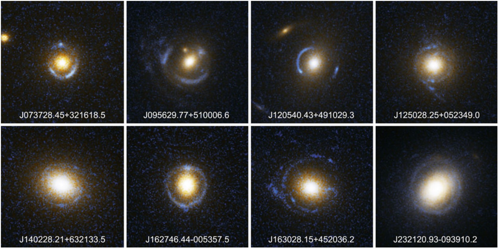
Figure 3: Examples of strong lens systems that produce arcs and Einstein rings. Figure from Reference [3]

Systems that exhibit strong gravitational lensing resulting in Einstein rings are probably the easiest of the scenarios to analyze. Astronomers measure the Einstein radius, usually in units of arcseconds, and use spectroscopy to measure the redshift of the source and lens, if it is visible, to determine the mass of the lensing object.

2.3 Weak Gravitational Lensing

Weak gravitational lensing is significantly less obvious than strong gravitational lensing, and usually requires a more statistical approach to determine if an object is being lensed. Telescopes are aimed at clusters of galaxies in order to observe as many objects as possible. Individual galaxies are elliptical, but the average shape of a large collection of random galaxies should be circular. Thousands or even tens of thousands of galaxies are monitored for months at a time in order to precisely determine their shape. The change in ellipticity of the averaged galaxy shape is just a small fraction of a percent, requiring sophisticated imageanalysis algorithms to recognize. This distortion is quantified in terms of tangential shear $(\gamma_t)$ . For our purposes here, tangential shear is the same as the ellipticity, defined as

(12) $\begin{equation*} e = (a-b)/(a+b),\end{equation*}$

where $a$ is the major axis and $b$ is the minor axis of the ellipse. Researchers monitor the magnitude of this distortion as a function of radius of the expected lens to produce datasets like the one shown in Figure 4.

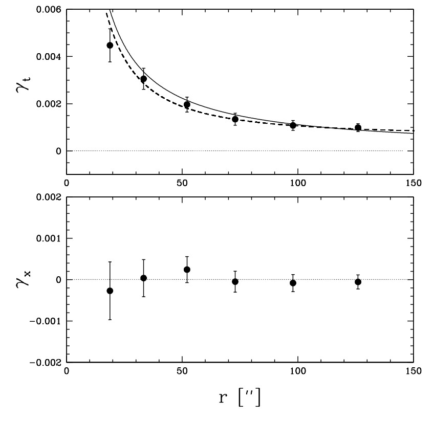
Figure 4: The top plot is an example of the changes in tangential shear as a function of distance across a lensing object. The solid line is the best-fit isothermal sphere. The dashed line is a more complicated fit with a parameter-dependent density profile describing the galaxy. The x-axis is the radial distance in units of arcseconds. The bottom plot shows the signal with the source images rotated by 45^◦. This signal is called the cross-shear, and is expected to be consistent with zero if the cause of the distortion is gravitational lensing. Figure from Reference [4]

Extracting the mass of the lensing object from such a dataset requires assumptions about the lensing object. If the object is a galaxy, which is frequently the case, then one would require knowledge about the ellipticity of the galaxy and its mass profile. A good approximation is to assume that the galaxy is an isothermal self-gravitating gas cloud. In such a model, the tangential shear is proportional to the Einstein angle [4]:

(13) $\begin{equation*} \gamma_t = \cfrac{\theta_E}{2\eta}. \end{equation*}$

2.4 Gravitational Microlensing

Microlensing is the smallest of the three gravitational lensing affects. As discussed in Section 2, a gravitational lensing event is always associated with a magnification of the source object. Objects that are gravitationally microlensed display a characteristic light curve like the one in Figure 5. As the lens passes in front of the source, the source is magnified, resulting in an increase in detected light. Note that the observation of this light curve alone is not enough to definitively identify a gravitational lensing event. Researchers compare light curves in different colours to be sure that the signal is achromatic, as one would expect if the cause was gravitational lensing since it affects the entire electromagnetic spectrum in the same way.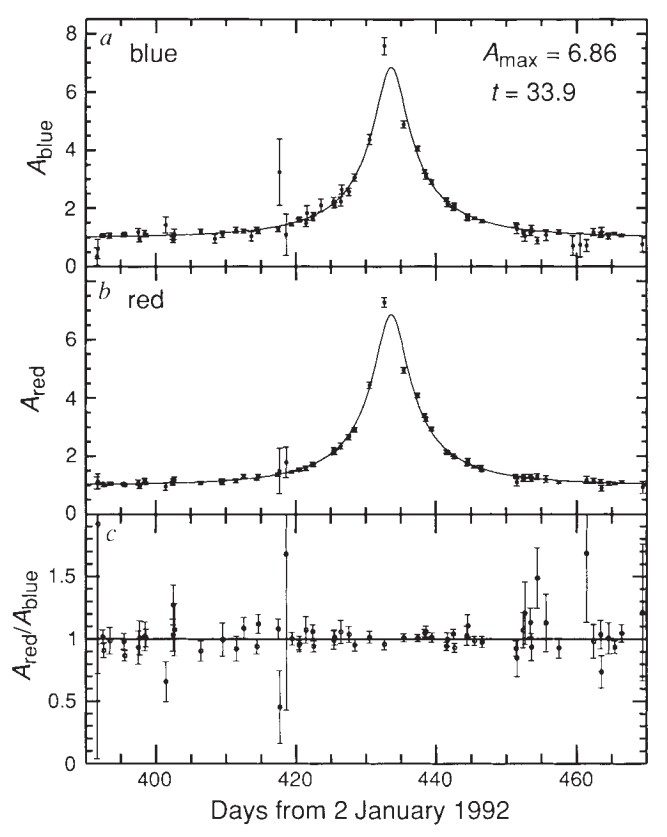

Figure 5: An example of a light curve that results from the changes in image magnification during a microgravitational lensing event. Details of the fit are discussed in the text. Figure from Reference [7]

Microlensing is used to find incredibly small lenses. These objects are incapable of even changing the shape of the source image, and only result in changes in apparent brightness. As opposed to strong and weak gravitational lensing, which are used to study galaxies and clusters of galaxies, microlensing experiments search for star or even planet-sized lenses [7].

The characteristic time-scale of this variability is given by

(14) $\begin{equation*} t_E = \cfrac{\theta_E}{\dot\theta}, \end{equation*}$

where $\dot\theta$ is the angular velocity of the lensed image. This time scale is typically on the scale of a month for commonly lensed objects. It is difficult to describe how incredibly coincidental this result is for us Earthly observers. If the transit of the lens took much longer, there would be annual gaps where the object is not visible, while much shorter variations would be difficult to observe. It is also worth noting that microlensing events, like most other gravitational lensing events, are one-time-only events.

We define the position of the source in the source plane as

(15) $\begin{equation*} y(t) = \sqrt{p^2+\left(\cfrac{t-t_{\text{max}}}{t_E}\right)^2},\end{equation*}$

where $y=\beta/\theta_E, p$ is the minimum distance from the optical axis (i.e. $\eta_\text{min}$ ), and $t_\text{max}$ is the time $t$ at which $y=p$ , and the magnification reaches its maximum value. The light curve then has the form

(16) $\begin{equation*} S(t) = S_0(t) = S_0\cfrac{y^2(t)+2}{y(t)\sqrt{y^2(t)+4}}.\end{equation*}$

$t_\text{max}, t_E,$ and $p$ are all measurable from a light curve, but $t_\text{max}$ and $p$ are terribly uninteresting and provide no information about the lensing object. Since $t_E \propto \sqrt{MD_L}/v$ , one can derive the mass of the lensing object only if the lens velocity and distance is known, otherwise astronomers must settle for a measurement of the combination of those variables.

Introduction

2.1 Gravitational Lensing Formalism

2.2 Strong Gravitational Lensing

2.3 Weak Gravitational Lensing

2.4 Gravitational Microlensing

License

Share This Book