Laser Beam Profile
Introduction
3.1 Laser Beam Profile
You are probably familiar with ray optics where light is drawn as rays that can be focused perfectly. In reality, the most ideal laser beam we can generate is ‘diffraction-limited’, meaning that the diffraction of the light due to it passing through an aperture (like the face of the laser housing) limits how small the radius of the beam can be. The result is the so-called Airy disk, shown in Figure 1. Note the constructive and destructive interference, akin to the diffraction pattern of the famous double-slit experiment. The intensity of the center peak of the Airy disk is described by the Gaussian function, which will not be written here since you should be able to write that function in your sleep by now.
An image of a propagating laser beam is shown in Figure 2. An important parameter in discussing laser beams is the beam divergence, defined as  in Figure 2. Due to the assumption that the beam is diffraction limited, the beam divergence and beam waist (
 ) are not independent. They are forced to obey the following equation:
(1) 
where  is the wavelength of the light. Rearranging the equation, we see that
(2) 
Therefore, a very small beam waist can only be achieved with a very large divergence, and vise versa; limited by the wavelength of the light.
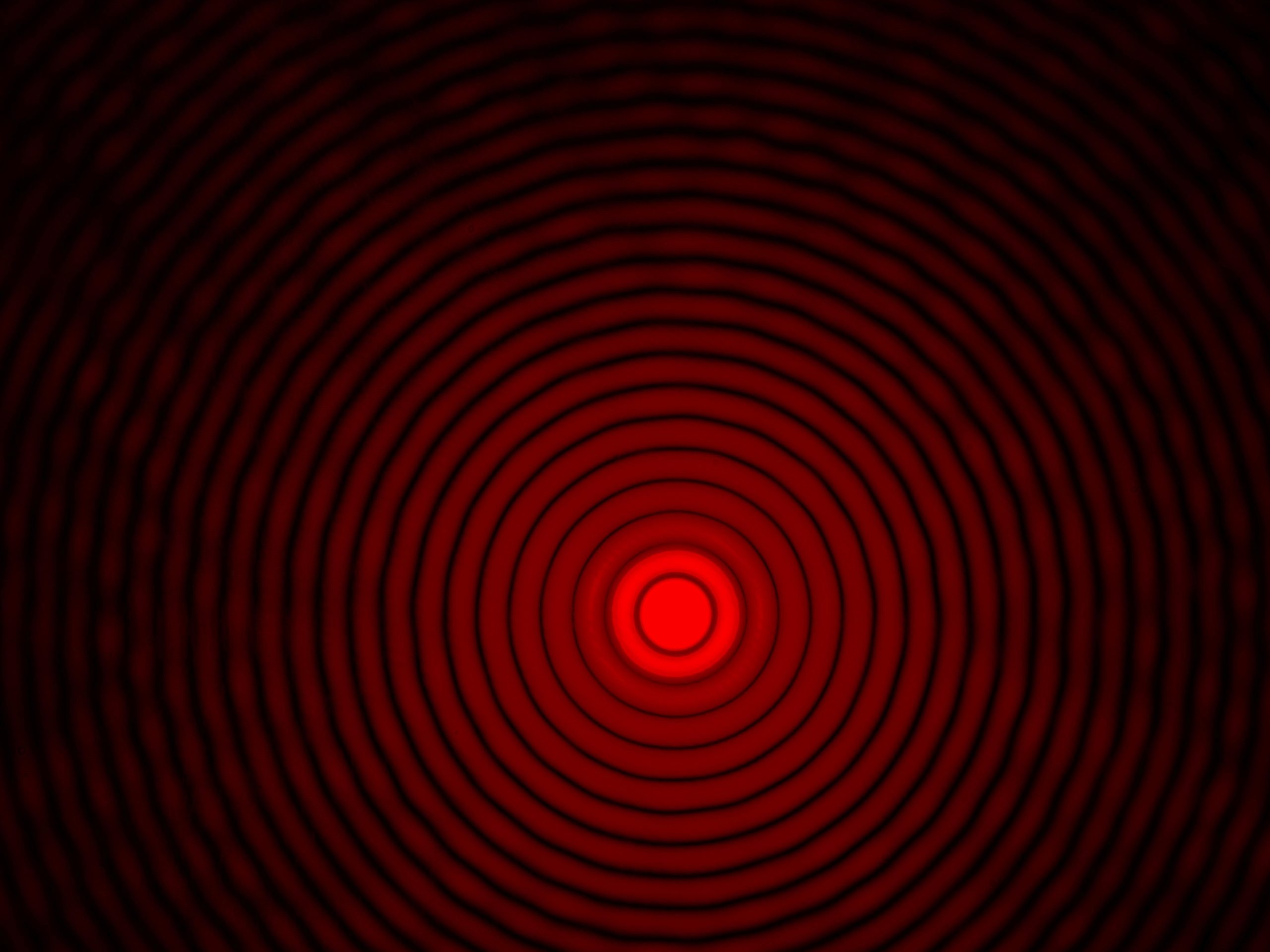
Figure 1: An Airy disk that results from a He-Ne laser passing through a pinhole. Note that you will not see this many rings in your experiment. Image from Wikipedia.
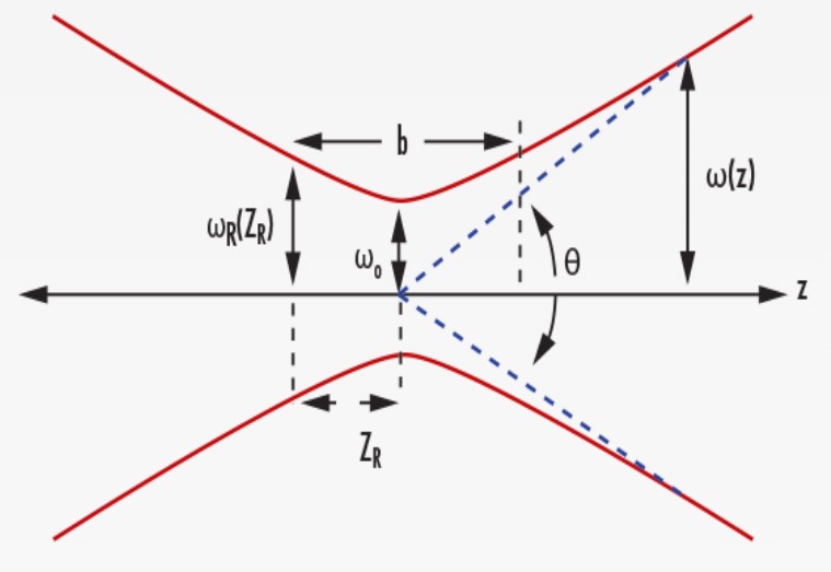
Figure 2: Schematic of a laser beam profile.  and are the only relevant variables for this experiment.
3.2 Laser Beam Profile Measurement
Laser beam profiles are typically measured by sweeping an edge across the face of the beam and measuring the intensity of the partially-blocked beam as a function of the radius. The result is the integration of the Gaussian beam profile, which as we all know, is the error function:
(3) 
This general form of the error function is missing some of the variables that we need in order to include the physics involved in this experiment. The following equation will allow you to fit your data and determine the width of the Gaussian beam profile:
(4) 
Where  is an amplitude term that is proportional the full power of the beam,
  is the error function (i.e. integrated Gaussian function),
  is the position of the beam, is the width of the beam (measured from
  of the peak intensity), and
  is an offset term since the center of this error function is not at the origin.
It is VERY important to note that in laser physics, the width of the beam is NOT the full width at half maximum (FWHM), but instead the width out to  of the peak, as in Figure 3.
Therefore, a very small beam waist can only be achieved with a very large divergence, and vise versa; limited by the wavelength of the light.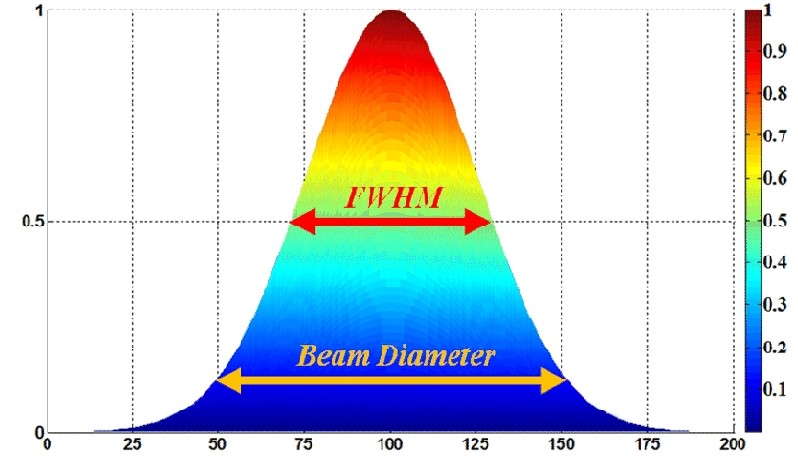
Figure 3: Beam waist measurements using the full width at half max (FWHM) and the beam diameter (). Figure from Wikipedia.
3.3 Beam Expander
3.3.1 Lenses
A beam expander is made of two lenses with different focal lengths, as in Figure 4. The magnification power (MP) is defined as
(5) 
where  is the focal length of the objective lens and
  is the focal length of the image lens, as in Figure 4. MP can also be expressed as ratios of beam width and divergence:
(6) 
Note that MP for a beam expander is less than 1 since the beam is being enlarged, not magnified.
By placing the image lens one focal length from the objective lens’ focal length, the output of the beam expander will be collimated, with a new diameter determined by MP.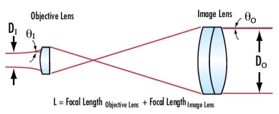
Figure 4: A schematic of a beam expander with relevant variables defined. Figure from Edmund Opticss.
3.3.2 Pinhole Diffraction
An ideal laser will produce a beam with an Airy diffraction pattern, but most lasers aren’t ideal – there’s some manufacturing imperfections or lens aberration that results in an imperfect beam. One solution is to add a pinhole to the beam expander at exactly the focal point of the first lens. When aligned correctly, the result is always an Airy disk with a Gaussian profile.