Introduction

Daniel FitzGreen

Radioactive Halflives

Introduction

3.1 Radioactive Decay

Unstable radioactive nuclei decay into a more stable state by emitting radiation such as electrons and positrons ( $\beta^-$ and $\beta^+$ particles), alpha particles (helium nucleus), neutrinos, and photons (often referred to as gamma rays). The probability that a nucleus will decay in a certain time interval does not depend on the state of chemical combination, the temperature, pressure, or the presence of other atoms or nuclei. There are some exceptions to the above statement when radioactive decay involves the interaction of the nucleus with its orbital electrons, but this effect is very small indeed. The rate of radioactive decay of a given sample is proportional only to the number of nuclei present, since radioactivity is a property of isolated nuclei. For a sample containing $N$ nuclei, the rate of decay is given by:

(1) $\begin{equation*} -\cfrac{dN}{dt}=\lambda N,\end{equation*}$

where $\lambda$ is the decay constant that is specific to the radioactive species. Integrating the above equation yields:

(2) $\begin{equation*} -\ln N = \lambda t + C,\end{equation*}$

where C is the constant of integration, and ln is the natural logarithm ( $\log_e$ ). If $N_0$ (the number of nuclei at $t= 0$ ), then:

(3) $\begin{equation*} -\ln N_0 = C \end{equation*}$

,

which leads to:

(4) $\begin{equation*} \cfrac{N}{N_0} = e^{-\lambda t} \end{equation*}$

The halflife, usually written as $t_{1/2}$ , is the time for one half of the initial number of nuclei to decay, so

(5) $\begin{equation*} \cfrac{N_{t_{1/2}}}{N_0}=\cfrac{1}{2} = e^{-\lambda t_{1/2}} .\end{equation*}$

A simple equation for the halflife follows:

(6) $\begin{equation*} t_{1/2} = \cfrac{1}{\lambda}\ln 2 = \cfrac{0.693}{\lambda} \end{equation*}$

The halflife of a given radioactive isotope is measured by monitoring the rate of radioactive decay as a function of time. The decay rate over time can be plotted on a semi-log plot. The result ought to be a straight line, the slope of which is the decay constant $\lambda$ , which is used to determine the halflife.

In many cases, a radioactive sample will contain two or more radioactive substances with different halflives. If the radiation detector responds to the rays emitted by each component, then the decay curve will no longer be a straight line. For two components, if the two halflives are sufficiently different, the shorter-lived component will decay almost completely while a substantial amount of the longer lived component remains. Such a situation is shown in Figure 1.

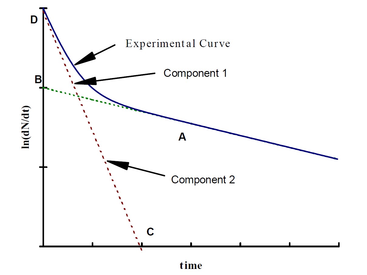
Figure 1: An example plot of detector count rate vs time. The solid line shows the count rate of the detector. The dashed line shows the contribution from each component of the sample.

Beyond the point A, the decay curve is almost a straight line, which may be extrapolated backwards, as shown, to determine the decay rate due to component 2 at earlier times. The line AB then represents the logarithm of the contribution of component 2 to the mixture. This contribution may be subtracted from the experimental curve, yielding a straight-line CD, which represents the contribution due to component 1. Remember that you are dealing with the logarithms of the count rates and that taking their difference directly from the above curves is equivalent to taking the ratio of the two rates, not the difference.

3.2 Poisson Statistics

The Poisson distribution is a discrete probability distribution for the counts of events that occur randomly in a given time interval. The Poisson distribution lends itself well to counting experiments, where ionizing radiation is produced randomly from the decaying isotope. The probability of observing x events in each interval is given by

(7) $\begin{equation*} P(X = x) = e^{-\lambda}\cfrac{\lambda^x}{x!},\end{equation*}$

where $X$ is the number of events in a given time interval, and $\lambda$ is the mean number of counts per time interval. One can succinctly write $X \sim Po(\lambda)$ , and say that $X$ follows a Poisson distribution with parameter $\lambda$ . If $X \sim Po(\lambda)$ , then it can be shown that $\theta = \sqrt{\lambda}$ . In the context of this experiment, the mean counts per unit time is what is recorded as you monitor the isotope decay, and the square root of the mean number of counts is the uncertainty in that mean count.

Introduction

3.1 Radioactive Decay

3.2 Poisson Statistics

License

Share This Book