Gravitational Lensing
Experimental Apparatus
As one could imagine, an actual measurement of a gravitational lensing object is quite time consuming. The observer must monitor literally millions of stars for months and constantly analyze data in search of the key indicators of a gravitational lens passing in front of an object. We only have a three-hour session, so completing an actual gravitational lensing measurement is not realistic. Instead, we will use acrylic lenses that have been machined to emulate the way a gravitational lens bends light.
A digital camera, lens mount, and backdrop are mounted on a linear rail on the benchtop, as shown in Figure 4. The user can control the distance between all of the components on the rail and measure with the ruler on the side of the rail. Images can be saved from the camera using the Python script run from the PC and analyzed with ImageJ.
3.1 Lens Details
The details of the lens construction are contained in Reference [1]. You don’t necessarily need all these details in order to do this experiment, but it’s still pretty neat! Basically, Snell’s Law is used to relate the deflection through the lens to its thickness, arriving at a differential equation for the lenses thickness:
(7) 
As discussed in Section 2, the deflection angle for a point mass is  . The deflection angle of more interesting, and more realistic, objects can be described by integrating their mass as a function of
(8) ![\begin{equation*} \text{constant density sphere: } M \left[ 1 - \left( 1 - \cfrac{\xi^2}{R^2}\right)^{3/2}\right],\end{equation*}](https://ecampusontario.pressbooks.pub/app/uploads/quicklatex/quicklatex.com-f0f51a1cf80d6ed6ad04fa54d0c70b05_l3.png "Rendered by QuickLaTeX.com")
(9) ![\begin{equation*} \text{isothermal gas cloud: } M \left[ 1 - \left( 1 - \cfrac{\xi^2}{R^2}\right)^{1/2} + \cfrac{\xi}{R}\cos^{-1}{(\cfrac{\xi}{R})}\right], \end{equation*}](https://ecampusontario.pressbooks.pub/app/uploads/quicklatex/quicklatex.com-e11480942033f31d58752553ba9fe4d7_l3.png "Rendered by QuickLaTeX.com")
where  is the total mass of the object and
  is the radius of the object. Note that when
  , the mass distribution is that of a point mass.
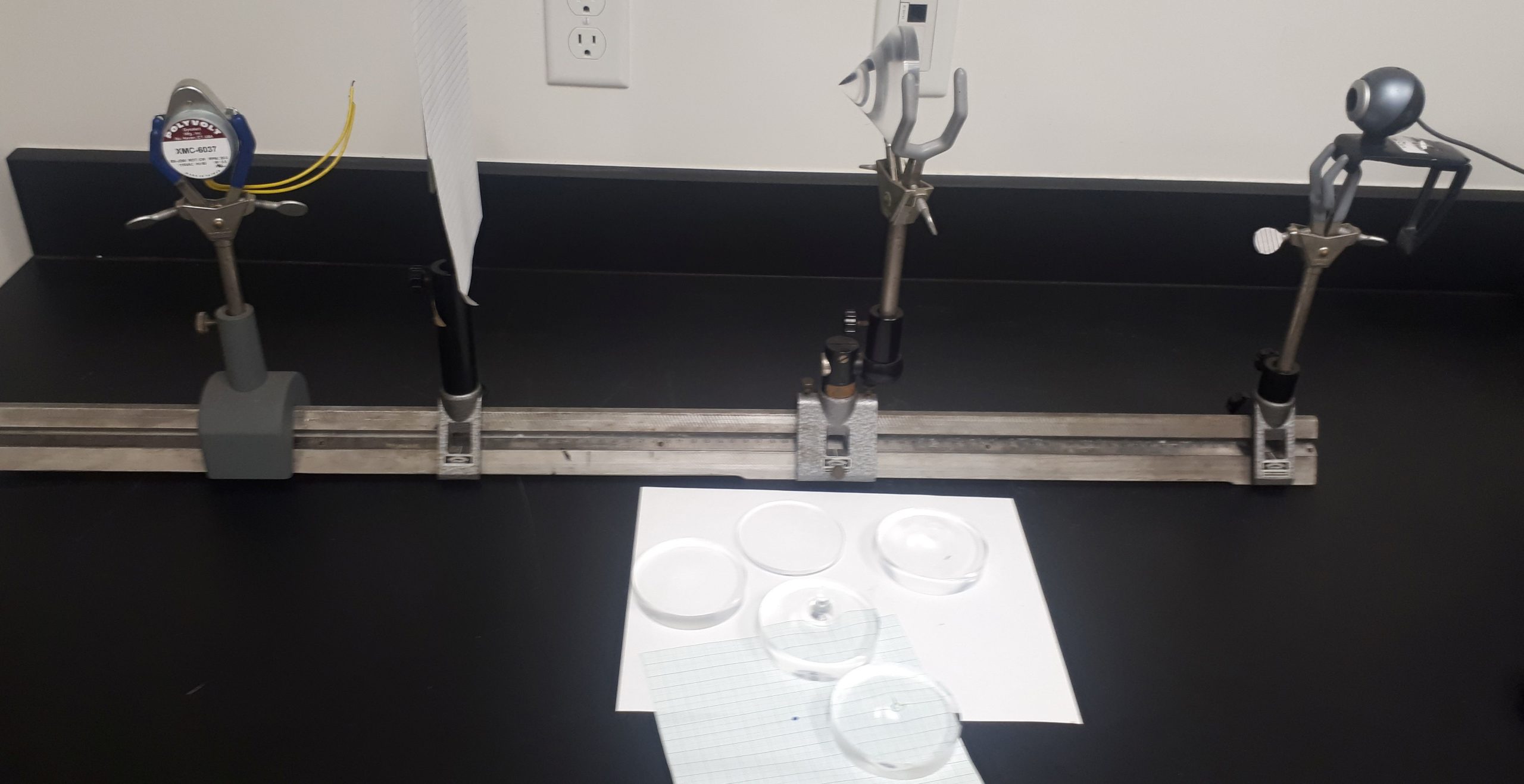
Figure 4: Gravitational Lensing apparatus on the benchtop.
The lens thickness for a point mass lens given by Equation (7) is then:
(10) ![\begin{equation*}T(R) - \cfrac{4GM}{c^2(n-1)}\ln\left[ \cfrac{\xi}{R}\right] \end{equation*}](https://ecampusontario.pressbooks.pub/app/uploads/quicklatex/quicklatex.com-adee9404a4cff363d89d3fbdf75510cb_l3.png "Rendered by QuickLaTeX.com")
where  is the index of refraction of the lens material (usually around 1.49 for acrylic).
  is the thickness of the lens at the boundary of the object, and is the constant of integration that falls out of Equation (4), which lets us choose the total thickness of the lens.
3.2 Image Recording & Analysis
A Python program using OpenCV displays the webcam image, and allows the user to record frames. For measurements of the Einstein radius, the program is simply used to record a frame from the webcam for analysis with ImageJ.
ImageJ is a free image-analysis software suit you can download. The images from the webcam may not have the level of contrast required to see how the images are distorted. Users can enhance the contrast of
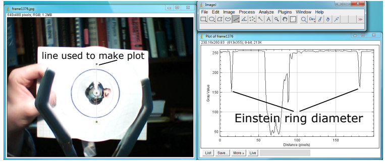
Figure 5: An example analysis of an Einstein ring using ImageJ.
their image under ‘Process’→‘Enhance Contrast…’. If the image contrast can be increased enough, the user draw a line through the relevant section of the image and create a ‘Plot Profile’ under the ‘Analyze’ menu. The plot profile should make it easier to make a precise determination of the Einstein radius. An example of an Einstein ring analysis is shown in Figure 5.