4.1 Radiation Detector

The decay of the radioactive isotopes will release radiation with a spectrum of energy. The radiation is detected using a Geiger-Mueller (GM) tube. A GM tube contains a mixture of gas that contains an inert gas like helium, argon, or neon, and an anode wire. A high voltage is applied to the wire – usually around 1 kV. Incoming radiation ionizes the inert gas, and the electric field from the applied high voltage attracts ionization-electrons towards the wire. If the electric field is high enough, The electrons gain enough energy to ionize more gas atoms, creating an avalanche affect. Due to how the initial ionizing radiation is detected and amplified, a GM tube cannot be used as a spectrum analyzer – the GM tube cannot discriminate between radiation types or energies.

The operating voltage of a GM-tube typically has three stages: a proportional counting region, a plateau region, and a glow discharge region, as shown in Figure 2. In the proportional region, the electric field from the high voltage is not large enough to cause a complete discharge along the anode. Increasing the voltage will increase the number of discharges in the GM tube, thereby causing a substantial change in the number of detected counts. At higher voltages, the gas around the anode is completely ionized, so small changes in operating voltage do not change the number of radiation particles detected. At even higher voltages, the electric field alone ionizes the inert gas without any radiation catalyst. Clearly, one should avoid operating a GM tube in this region. At very high voltage, electric arcs can occur between the anode and the GM tube wall, damaging the anode wire and rendering the GM tube useless (unless you really, really like paperweights).

This experiment uses a Spectrum Techniques ST360 controller and N2101BNC GM tube from St. Gobain. The ST360 automatically discriminates (i.e. doesn’t count low-energy background radiation) and counts pulses from the GM tube. Computer software controls the GM tube high voltage, displays the number of counts, and can be automatically programmed to repeatedly count radiation over a long monitoring period.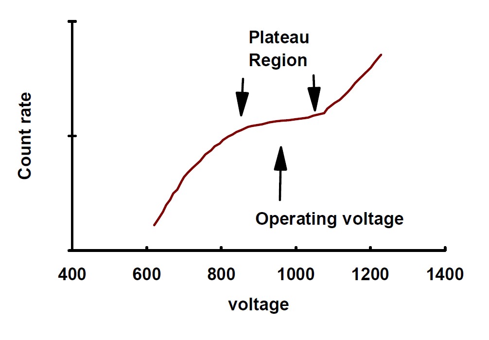

Figure 2: An example plot of the GM tube count rate as a function of operating voltage.

The program provides basic control and display features (see the accompanying notes in ST360 manual). You can set the number of data points to acquire and the sample time interval between data points. A timer in the ST360 accurately measures the sample interval. (How might you verify this?) The data is displayed in both a table format and a graph.

A non-negligible amount of time passes between when an ionizing radioactive decay particle passes through the detector, and when it creates an electron avalanche, the detector electronics register the count, and the electronics are reset to detect the next decay particle. This minimum time between possible successive counts is called ‘dead time’, and it becomes very relevant at high count rates. This experiment already has a lot of new physics for a 2^nd year student, so this correction will be ignored for now, and explored in the 3^rd year labs.

The rate of coincident pulses in the Geiger tube can be thought of as the product of the fraction of all time which lies within the resolving time of any pulse (, which is assumed to be  1 s) and the rate of pulse arrival () or

(8)  

where is the true rate, is the measured rate and  is the resolving time.

Since coincident pulses are likely to be counted as one, the measured rate will be reduced from the true rate by the coincidence rate:

(9)  

Solving for gives the true rate at which radiation is passing through the detector:

(10)  

If the resolving time  is known, a correction to your measured rate can be calculated using the above formula. Depending on the size and type of the detector, the resolving time can be microseconds to milliseconds. The resolving time is given by

(11)  

where the variables are explained in Section 5.3.

4.2 McMaster Nuclear Reactor

The sample that is used in the final parts of the experiment is irradiated in the McMaster Nuclear Reactor (MNR). The reactor is an open-pool type reactor, where the core is clearly visible from above. If you ever get the chance, take a tour of the reactor. It’s free, interesting, and a great date-night! The RABBIT system, which is a system of pneumatic tubes, pushes the sample from the input in the high level labs, to a position just beside the reactor core. The sample is irradiated for a specified amount of time, then sent back to the output in the high level labs.