Part 2: Discharging through an LR Circuit

nejatsm

Part 2: Discharging through an LR Circuit

Using Circuit_2 with $R = 10 \Omega$ and an initial voltage of 1 V, we are going to apply linear regression to a current versus time curve. This will allow us to calculate the inductance from the slope of the line of best fit.

PROCEDURE

1. Create a Voltage versus Time and Current versus Time graph on Capstone. Your Capstone should already have these set from the previous part.

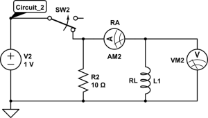
2. Construct Circuit_2 exactly as shown above with the following settings:

a. Waveform = DC.

b. DC Voltage = 1V.

c. Set the frequency of measurement to the “Common Rate” of 1 kHz (this will record a value for voltage and current every millisecond).

3. Once your circuit is made, with the switch set to CLOSED, turn on the power supply and start recording. After a few seconds (<2s), OPEN the circuit and stop recording a few seconds after.

a. Note: Capstone has trouble tracking large amounts of data, so chances are it will automatically stop recording after about 6s.

4. Copy your voltage versus time and current versus time graphs from Capstone and add them to the report.

5. Now we are going to take the data and prepare it for linear regression.

a. Remove every data point that is at $\mathbf{I_0 = \frac{V_T}{R_A + R_L}}$ besides the last one. This last data point will be your initial time $\mathbf{t_0}$ so record its value in the report. To remove some data from your graph:

i. Select the option “Highlight range of points in active data” (this icon looks like a series of highlighted points) and cover the highlighted box over the desired data to be deleted. You can move and resize the box as needed. Then right click the highlighted box and select “Deletions $\rightarrow$ Delete Highlighted Data Points”.

b. Remove every data point that is after $\mathbf{t_0 + 2 \tau}$ . Use the average value of you previously calculated for $R=10 \Omega$ .

CHECKPOINT

(Ask the TA to check your graph for the appropriate data range)

Export the data for this graph and import it into Excel. To do this:

a. Select “File” tab within Capstone and then “Export Data…”. The data file generated should automatically be in a comma separated value (CSV) format.

b. Select “Export to file” in bottom right corner. Name the file an appropriate name and save it to your local directory (folder).

c. Right click on the csv file you just saved. Then go to “open with” “Microsoft Excel”.

7. Create a plot of $\mathbf{ln (I)}$ versus time for a domain of $\mathbf{t \in [t_0, t_0 + 2 \tau] }$ from the loaded data in Excel. There are multiple ways to do this, but the easiest is to:

a. Click the “Insert” tab $\longrightarrow$ “Charts” $\longrightarrow$ “Insert Scatter (X,Y) or Bubble Chart)” $\longrightarrow$ “Scatter”.

b. Right click the empty graph, select “Select Data” $\longrightarrow$ “Add”.

c. Left click under “Series X values:” $\longrightarrow$ highlight the time column. Likewise, do this for the “Series Y values:” for the natural logarithm of current column.

Caution: For time, you need to write every value with respect to $\mathbf{t_0}$ since that is where the exponential decay started.

8. Give your plot a title and appropriate axis labels. To do this:

a. Left click anywhere on the graph, select “Chart Design” tab, then select “Add Chart Elements”.

9. Insert a trendline on the graph and display the equation & value on the graph. To do this:

a. Right click the data series in the graph, select “Add Trendline…” $\longrightarrow$ “Display Equation on chart” $\longrightarrow$ “Display R-squared value on chart”.

10. Use the slope of the trendline you just found, along with Equation (8) to determine the inductance and time constant of your circuit. Add your plot to the report. Make sure your plot has properly labelled axes and titles.

The theory tells us that the current for Circuit_2 is given as

$I(t) = I_0 e^{-\frac{R_T}{L}t},$

which gives a natural logarithm of

(8) $\begin{equation*} ln (I(t)) = - \frac{R_T}{L} t + ln (I_0). \end{equation*}$

The value of $\tau = \frac{L}{R_T}$ should remain the same as well.

Question 4

How do the voltage and current versus time plots behave in the $t rightarrow t_0$ and $t \rightarrow \infty$ limit? Compare this to the plots found in the previous part.

Question 5

Based on your plot of current versus time, how long does it take for the inductor to discharge to 36% of its original current? If we didn’t consider the internal resistance of our circuit elements, the time constant would be expressed as $\tau = \frac{L}{R}$ . How would having this new time constant change the current and voltage versus time plots?

Question 6

From the slope of your line of best fit, calculate the inductance and the time constant. How close are these values to the previous ones found in part 1 with $R = 100 \Omega$ ? Justify why you think these values are more accurate compared to the previous ones.

Question 7

(Challenging) By the end of this lab, hopefully you have come to realize just how important internal resistance can be when analysing the results of any circuit. It often tends to compound itself, leading to unintuitive outcomes. What other sources of internal resistance could be affecting the outcome of our results, and how might we go about modelling its behaviour? Given the resistors we use are on the order of $10 \Omega s$ , would these extra internal resistance values ultimately change the outcome in a meaningful manner? Finally, why wasn’t internal resistance considered in the other labs in Physics 1E03 (should it have been)? Explain.

Part 2: Discharging through an LR Circuit

PROCEDURE

CHECKPOINT

License

Share This Book