THEORY
INDUCTORS
Inductors, like capacitors, are circuit elements used to store energy. However, where capacitors store energy in the form of an electric field, inductors use a magnetic field. When a current travels across a conductor (like a wire), a magnetic field is created around the wire. By bending the wire into a loop, the magnetic field’s direction can be made to pass through the middle of the loop. By combining multiple loops (like winding a wire around a tube), the magnetic field within the tube can be increased as the field created by individual loops combine. An inductor is essentially a wire-wrapped tube.
Inductors are characterized by their inductance,  , which has units of Henrys. Henrys are a measure of the magnetic flux
  an inductor can maintain divided by the current required to create the magnetic flux,
  i.e.
i.e.
![\[L = \frac{\Phi}{I}.\]](https://ecampusontario.pressbooks.pub/app/uploads/quicklatex/quicklatex.com-43cab252785c044006010a3fea4cd101_l3.png "Rendered by QuickLaTeX.com")
Magnetic flux is the “amount” of magnetic field passing through a surface and has units of [ ]. So a Henry is equivalent to [
 ] in SI units. However, since the magnetic flux through the inductor is so closely related to the geometry of the wire loops, the inductance of an inductor can be calculated by considering how the inductor is made:
![\[L = \mu \frac{N^2 A}{L}\]](https://ecampusontario.pressbooks.pub/app/uploads/quicklatex/quicklatex.com-f60f6bf5aa29788e12b4c0baf8eddaea_l3.png "Rendered by QuickLaTeX.com")
where N = the number of wire turns, A = cross-sectional area of the inductor, L = length of the inductor, and  is a constant related to the permittivity of the space within the coils.
When a circuit containing an inductor is initially turned on, the immediate input of current causes a quick change in magnetic flux through the inductor. When there is a change in magnetic flux, an “electromotive force” or emf (ε) is generated:
(1) 
This emf is a voltage that opposes the applied voltage, effectively resisting the applied current. As the inductor builds its magnetic field, its induced emf decreases until the inductor reaches a steady-state magnetic flux. At this steady-state, the change in flux is zero, and the induced emf is also zero, which means the resistance the inductor produces goes to zero as well. When the voltage source is removed, the magnetic flux through the inductor will decrease again. Now, an emf is generated in the opposite direction (the original direction of the applied voltage).
SERIES RL CIRCUIT
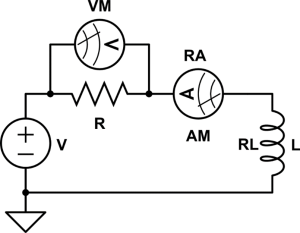
Figure 1: Series RL circuit with internal resistance of the ammeter and inductor included.
The series RL circuit behaves very similarly to RC circuits in that the current and voltage are time-dependent. That is, the voltage and current passing through different sections of the circuit change with time. We will be exploring how this circuit behaves within this lab and we will be considering the internal resistance of both the ammeter and inductor.
We can characterize the voltage by using Kirchhoff’s voltage law and Ohm’s law. The voltage of the circuit will be
(2) 
where  is the internal resistance of the ammeter, and
  is the voltage across the inductor. has two components, one from the emf generated by the inductor (Equation 1) and another from its internal resistance (through Ohm’s law). We can characterize the inductor’s voltage as
(3) 
Combining equations (2) and (3), we get a first order differential equation as
(4) 
where  or the total resistance of the series circuit. You can solve equation (4) by substituting an integrating factor in the form of
![\[\frac{d}{dt} \left( e^{\frac{R_T}{L} t} I \right) = \frac{V}{L} e^{\frac{R_T}{L} t},\]](https://ecampusontario.pressbooks.pub/app/uploads/quicklatex/quicklatex.com-c63ccea32a3b6c2b6c4277d192e2ba61_l3.png "Rendered by QuickLaTeX.com")
![\[\Rightarrow I(t) = \frac{V}{R_T} + C e^{\frac{R_T}{L} t}.\]](https://ecampusontario.pressbooks.pub/app/uploads/quicklatex/quicklatex.com-ae779510aa775756e9284ce15910c796_l3.png "Rendered by QuickLaTeX.com")
We can use the initial condition that  to solve for the constant
  and get
(5) 
When looking at equation 5 , we can determine a time constant for our circuit in a similar manner to Lab 3. The time constant is defined as the amount of time it takes the current to decrease by (  )
)  or by 63.2%. The quotient of
  has units of seconds when R is in
  and L is in Henrys (you can check this for yourself) and is called the time constant of the circuit.
So the time constant for the RL circuit, including internal resistance, is given as
![\[\tau = \frac{L}{R_T}.\]](https://ecampusontario.pressbooks.pub/app/uploads/quicklatex/quicklatex.com-bcf116dc8307ca77321095e9a272fde3_l3.png "Rendered by QuickLaTeX.com")
If we didn’t consider the internal resistance of our ammeter or inductors within the circuit, the time constant would take a similar form as  .
.
Using Ohm’s law along with our result for the current, we can solve for the voltage across the resistor  as
as
(6) 
The important things to understand from equation 6 are the  and
and  limits which give
![\[lim_{t \rightarrow 0}~ V_R (t) = 0 ~\&~ lim_{t \rightarrow \infty } ~V_R (t) = V \frac{R}{R_T}.\]](https://ecampusontario.pressbooks.pub/app/uploads/quicklatex/quicklatex.com-0043a7f25ff05145c6f9754614141e73_l3.png "Rendered by QuickLaTeX.com")
We will be studying the RL series circuit experimentally and verifying equations 5 and 6 within Part 1 of this lab. If we didn’t consider any internal resistances within this circuit, the current would have a similar shape, but the voltage would take on a negative exponential which approaches zero as .
PARALLEL RL CIRCUIT
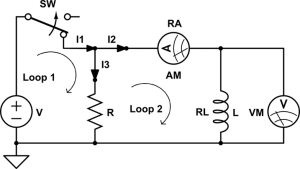
Figure 2: Parallel RL circuit with the internal resistance of the inductor and ammeter included.
Part 2 of this lab will involve using a parallel RL circuit. We will use this circuit to discharge the inductor through the resistor. So, the circuit will start off closed and then open at a time  . What we mean by this is that everything after the circuit opens will be measured from a time of zero.
Since we are only interested in what is going on in the inductor, we can focus on the loop which has the inductor in it. Assuming the inductor is fully charged, if we open the circuit, then the parallel RL circuit becomes that shown in Figure 3. Using Figure 3, we can write out Kirchhoff’s voltage law and get
![\[-IR - I R_A + V_L = 0,\]](https://ecampusontario.pressbooks.pub/app/uploads/quicklatex/quicklatex.com-2175d6dfa8ccc7152a6e14113afb8d3b_l3.png "Rendered by QuickLaTeX.com")
where  . This gives,
![\[\frac{d I}{dt} + I \frac{R_T}{L} = 0\]](https://ecampusontario.pressbooks.pub/app/uploads/quicklatex/quicklatex.com-02c8dbbe28b16d55263687b1fd75862d_l3.png "Rendered by QuickLaTeX.com")
where  . This equation can be solved separately by
![\[\frac{d I}{I} = - \frac{R_T}{L} dt,\]](https://ecampusontario.pressbooks.pub/app/uploads/quicklatex/quicklatex.com-d464463750d350ba5bca6a8d6c243098_l3.png "Rendered by QuickLaTeX.com")
![\[\Rightarrow I(t) = I(0) e^{-\frac{R_T}{L}t}.\]](https://ecampusontario.pressbooks.pub/app/uploads/quicklatex/quicklatex.com-6db590b4f93f2058abd4c78c8fea190c_l3.png "Rendered by QuickLaTeX.com")
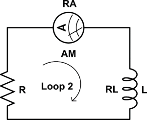
Figure 3: Examining the parallel RL circuit when the circuit is open.
By solving Kirchhoff’s voltage and current laws for Figure 2, we can get the initial condition for the current flowing the inductor (I2) as
![\[I(0) = \frac{V}{R_A + R_L},\]](https://ecampusontario.pressbooks.pub/app/uploads/quicklatex/quicklatex.com-e0aace0da3e88ba15d414537eb9baf1f_l3.png "Rendered by QuickLaTeX.com")
where we used the fact that the electromotive force of the inductor  at time
  (I encourage you to try and show this on your own). This along with equation 3 gives the result of
(7) 
We are going to again study this circuit experimentally and compare these theoretical predictions to the experimental results. For the voltage, the zero and infinity limit give
![\[lim_{t \rightarrow0} V_L(t) = V \left( \frac{R + R_A}{R_A + R_L} \right) ~\& ~ lim_{t \rightarrow \infty} V_L(t) = 0.\]](https://ecampusontario.pressbooks.pub/app/uploads/quicklatex/quicklatex.com-913f0b3c918c232130d96970c4386bef_l3.png "Rendered by QuickLaTeX.com")