Experimental Setup

Selecting Balls

In this experiment, you will be given three droppable balls. Measure their respective masses with the scale. Do not remove the tapes and the cardboards from the balls before measuring their masses. Record their mass values in the Results section of the Report along with a name in order to distinguish them from one another. These names should be self-evident and not anthropomorphized to any degree.

Make sure you note the geometry and material for each ball while clearly distinguishing which mass is associated with which ball. You will be graded on how well the TA can determine which ball was used for which set of data.

Detector Setup

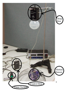
Your equipment for the experiment should already be set up upon your arrival. If it is not, please refer to the setup in Figure 1 and the instructions outlined in Appendix: Detector and Ball Setup.

Ball Setup

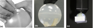
The balls should also already be set up for this experiment before your arrival. The key things to look for are a metallic end on one side of the ball (either a taped washer, or connected staple) as shown in Figure 2 (a), and a piece of cardboard attached to the other as shown in Figure 2 (c). If any of the balls you have chosen are missing these two key elements, please follow the setup instructions provided in the Appendix: Detector and Ball Setup.

Drop Box Setup

This setup is to ensure that the Drop Box is connected and working appropriately. Follow this procedure to ensure your Drop Box is working appropriately.

1.  Make sure the switch on the control box is set to Active.

2.  Suspend any of the chosen balls from their attached metallic (washer or staple) side to the Drop Box. Test all three balls you have selected to make sure they adequately attach to the magnetic end of the Drop Box. If any of your balls do not properly suspend from the magnet, please refer to the BALL SETUP section to ensure your chosen balls are properly arranged. If you are still having issues, call a T.A over to help with getting the balls properly set up.

3.  Adjust the Drop Box height so that the bottom of the ball is about 85 cm above the Motion Sensor input (gold). Note: You do not need to measure out exactly 85 cm with a ruler, this will be verified with the Capstone program later.

4.  Press the Timer Switch button and observe the falling ball. It should strike the Motion Sensor Guard directly above the Motion Sensor input. If not, adjust the position until it does. IMPORTANT: Do not drop any of the denser balls (golf ball, large plastic) onto the sensor without the guard as it may damage the motion sensor.

Capstone Setup

1.  In PASCO Capstone, set the Motion Sensor sample rate to 50 Hz (in the bar at the bottom of the window). Note that at this rate, the target ball cannot be more than one meter away. This frequency determines the number of data points you collect during the experiment. A graph of Position vs. Time will be loaded when you click on the Sensor Data tab. Hover near the top of the graph so that the Capstone tools pop up. Click on the “add new plot area” button (looks like an x-y axis) and add a second plot with Velocity on the vertical axis.

2.  We will also create another graph for the energy per unit mass as a function of time, which will include the potential energy per unit mass, the kinetic energy per unit mass, and the total energy per unit mass on the same plot, for each ball. This will complement the two other graphs we have in Capstone as well. Select the Capstone calculator option on the left-hand side. From there, explicitly type out the following commands for the various forms of energy per unit mass which all have units of J/kg:

‎                                       PE/m‎ = 9.8*[Position‎]

‎                                       KE/m‎ = 0.5*[Velocity]^2

‎                                       E/m ‎= [PE/m‎]+[KE/m]

Tip: If you type in the left square parenthesis  [  Capstone will automatically list the measurable quantities.

3.  After the energy values are entered in correctly, create a separate graph, which plots all three of these energies per unit mass on a single plot. To do this:

a.  Create graph of PE/m vs. Time. Left click the y-axis and select “Add Similar Measurement” to add KE/m and E/m to the vertical axis. This graph should show energy per unit mass for all three forms of energy on this same graph, with a legend on the right-hand side.

b.  You can change the y-axis label for the energy plot by left clicking “Custom Name” in the axis label position. Then select the properties button, which is in the tools bar at the top of the chart area. Change the Axis Label from there to “Energy/Mass” and click the “show custom label” button.

Note: At this point, you should have 3 plots, one is position vs. time, another is velocity vs. time, and the final plot is for the three energies per unit mass vs. time (Potential Energy is PE, Kinetic Energy is KE, and Total Energy is E).