Lab 6: Least Square Fitting
Lab 6: Least Square Fitting
Section 1:
First, we need to collect some data that you will need for your post-lab assignment.
On your lab bench there will be a power source attached to screws in a board, along with a voltmeter. The board includes two metallic strips in contact with the screws. When the power supply is turned on, these metallic strips resemble a capacitor – one side connected to ground and one side measuring the voltage set by the power supply.
Use a voltmeter to set the power supply to 3.00 V
DO NOT touch the board, except by the sides. DO NOT tape the board to the table. Lay the ruler carefully on the board without undue pressure and DO NOT drag it across the board.
Measure the potential at roughly 2 cm intervals. You will need to estimate uncertainties on position and potential. The specifications for the meter are on the table. (Hint: the uncertainty on the position is not strictly defined by the ruler specifications – take a look at the screw as well).
Use the big plastic rulers only.
Reading uncertainties on meters:
If the voltmeter gives me a reading of 6.00 V what is the uncertainty on this measurement? Use the data sheet for the voltmeter available in the Appendix – The Accuracy of a Multimeter.
Section 2:
Linear Regression
Last term, we considered uncertainties in the context of a single measurement, or repeated measurements of a single quantity. But often, theory predicts a relationship between two variables rather than the value of a single variable. If the relationship is linear, the standard approach to the problem is called linear regression, or least-squares fitting.
Exercise 1
You will be provided with a graph of a set of measured data, y vs x, for which theory predicts that y = mx+b. Of course, each measurement has an uncertainty of the kind we discussed last term, and so we would be surprised if all of the data fell onto a perfectly straight line! The question then becomes what line “best” defines the data (and for that matter, how is “best” defined?)
Download and open “LSF plot” in a software such as GIMP, Paint, PowerPoint, OneNote etc… You want a software where you can draw a line on the graph.
a) Draw a sensible line through the data.
b) Use the grid and scale to estimate the slope and intercept and write an equation which relates y and x.
Exercise 2
The standard way to design a best fit line is to minimize the sum of the squares of the deviations. Let’s see how well you did with your fit.
The data from Exercise 1 is in this Excel file that you can download.
a) Label column C of the spreadsheet: y calculated and use the equation of the line that you proposed in Exercise 1 to calculate the predicted value of y at each x. (It will save you some time in Exercise 3 if you put the slope and intercept into separate cells, and then build the linear equation with them as constants. Remember that to copy a constant from cell to cell, put a dollar sign in front of both the row and column, e.g. $G$1.)
b) Make a scatter plot in Excel which shows the actual data (as data points) and your line (as a solid line without markers).
c) Label column D deviation and calculate the difference (i.e. the deviation) of each measured y value from its predicted y value.
d) Label column E deviation^2, and calculate the square of each deviation.
e) At the bottom of column E, sum the squares.
Exercise 3
Now, Excel has a built-in function which will perform a least-squares analysis for you.
a) On your graph, right-click on one of the data points. Excel should provide you a menu of options, one of which is Add Trendline . Choose a linear fit and the options to display the equation on the chart, and to show R2.
b) Change the slope and intercept for the calculated y column to the values of your trendline and check the sum of the squares of the deviations for the Excel fit line. How does your line compare?
There are a number of assumptions built into the fit. The calculation assumes that the uncertainties on x are negligible compared to the uncertainties on y, that the uncertainties on y have a Gaussian distribution, and that all of the y values have the same uncertainty.
Exercise 4
a) You may have noticed (and been appalled!) that there were no uncertainties specified on the measured values. If the assumptions in exercise 3 are justified, then the measured deviations should be an indication of the uncertainty on each measurement. What might be a reasonable estimate of that uncertainty on each measurement?
b) In Excel, you can add error bars to a graph. If you click anywhere inside the graph, you should activate a Chart Tools menu. (Mine shows up at the very top of the screen. You might have to look around in your version.) Under Layout choose Error Bars. In this case, you should use either a Fixed Value or a Custom Value (it might be useful to understand how both options work) for all of the data points. (Use your estimate from part (a)).
Exercise 5
There is one important question left: what are the uncertainties on the best fit slope and intercept? (If the individual measurements have uncertainties, then surely any line fit to them will have uncertainties as well.)
In principle, you could estimate these by hand. You could look at your original graph, and ask: “What line could I put through the data that has a bigger slope but is still a reasonably good description of the data? What about a line with a smaller slope…?” Clearly there is room for variation since other students in the class (perhaps even at your table) came up with “best fit” lines that were different than yours. You could use these limits to estimate the uncertainty on the slope and intercept.
Excel has a function which will estimate the uncertainties on the slope and intercept for you. (The estimates come from the least squares argument using the assumptions described in Exercise 3. If you’re interested in the details of the argument, google.)
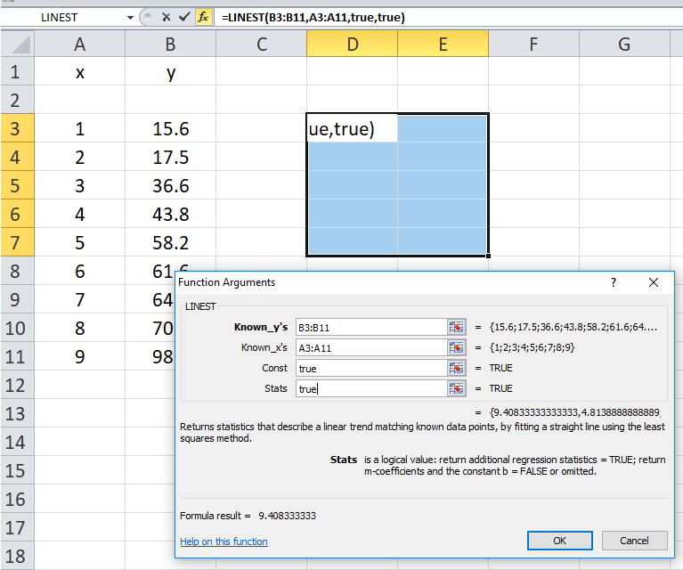
•Highlight a 5 x 2 block on the spreadsheet near your data.
•Click on fx and ask for the LINEST function.
•Fill in the query table with the required data (see the example below). Click OK.
•Highlight the entire equation in the equation bar (beside fx ) and press CNTL-SHIFT-ENTER. (Square curly brackets will appear around the function indicating that the output is an array. Mac users: you may have a different key combination. Google.) In the example below, D3 and E3 will be the slope and intercept: D4 and E4 will be their respective uncertainties. (The other cells are various statistical measures. Google if you’re interested…)
Congratulations on completing Lab 6!
Your post lab assignment is on the next page.