Lab 7: Calculating Electric Fields of Continuous Charge Distributions
Lab 7: Calculating Electric Fields of Continuous Charge Distributions
Exercise 1 – Discrete calculation with Excel
A thin rod lies along the x-axis as shown in the diagram below. It carries a total positive charge of 9 μC uniformly distributed along its length. Suppose that we would like to calculate the electric field created by the charged rod at the origin. (1 μC = 10-6 C)
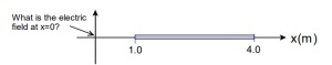
The only electric field that we know how to calculate exactly is the field of a point charge. Let’s start by estimating the electric field numerically on Excel as follows:
a) Break the rod up into 15 pieces of equal length, Δx.
b) In column A, Estimate the “position”, xi, of each piece using the x-coordinate of the centre of the piece.
c) Estimate the charge, Δqi, of each piece using the charge density at the centre of the piece and the size of the piece.
d) In Column B, estimate the electric field created by each piece at the origin using the point charge form
[latex]\Delta E_i = \frac{k\Delta q_i}{r_i^2}[/latex]
In a different cell, estimate the total electric field as
[latex]E \approx \sum_i \Delta E_i[/latex]
Exercise 2 – Continuous distribution and integration
The formal way to carry this calculation is to calculate an integral. Let’s first set it up carefully.
The goal is to calculate the field at x=0.
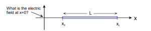
a) Draw the schematic
i) On the schematic, show a small segment, Δx in length. (It would be best to not choose a special piece (e.g. a piece at either end or in the middle.)
ii) If the rod carries a total charge Q, and has a length L, what is the charge density, λ, on the rod? In terms of λ, how much charge, ΔQ, is carried by that one little piece?
iii) How far is that piece from the origin? (Show it and label it on your diagram) Draw the field created by the piece of charge ΔQ.
b) Write an expression for the element of electric field at the origin, ΔE, created by that one segment and show the vector element on your diagram.
As you move from piece to piece along the rod, which, if any, of the variables in your expression change?
The electric field is then the sum of the fields from all of the pieces. In the limit where the size of the piece goes to zero, write an integral expression for the electric field at the origin. Think carefully about the limits of the integration.
c) Evaluate the integral expression for the rod in Exercise 1 and compare to your numerical estimate.
d) How would your derivation change if instead of calculating the field at the origin, you wanted to calculate it at x = 0.5 m? Rewrite the integral you would use to do the calculation.
e) How would your derivation change if instead of a uniform charge density, the density, λ, was given by λ = 2.0x C/m? Rewrite the integral you would use to do the calculation.
Exercise 3 – Another integral example
A thin rod of length 2L, carrying a uniform linear charge density, λ, lies along the x axis as shown in the diagram. What is the electric field at the point P, a distance y along the perpendicular bisector of the rod?
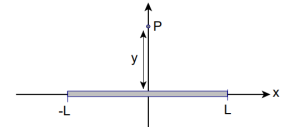
a) The electric field is a vector. Draw the electric field vector created by a piece of length Δx (that is not at x=0). In terms of λ, how much charge ΔQ is carried by a piece of length Δx?
b) In principle, you may have to calculate all three components of the electric field. For this reason, it is worth considering the symmetry of any problem before launching into a calculation. What would you expect the direction of the field to be at the point P? Why?
c) On the schematic, how far is that piece from the point P? (Show the distance on your diagram and label it r.)
Write an expression for the element of electric field, ΔE, created by that one segment and show the element on your diagram.
d) Clearly you are going to need to work by component and so you’ll need to introduce an angle, θ. It would be most convenient if you chose the angle so that the vertical component of the field was calculated as cos(θ). Label θ on your diagram.
e) Write an expression for the element of the relevant component of the electric field.
f) As you move from piece to piece along the rod, which, if any, of the variables in your expression change?
The electric field is then the sum of the fields from all of the pieces. In the limit where the size of the piece goes to zero, write an integral expression for the electric field at P.
g) At the moment, your expression for the electric field is probably technically correct, but you won’t be able to integrate it in this form – the differential is dx, but your variables are r and θ (which depend on x) and so you will need to rewrite the expression in terms of a single variable. In principle, you can choose any of r, x, or θ, but for this lab we’ll use θ.
Rewrite the expression in terms of the single variable θ and choose appropriate limits for your integral.
Post Lab Assignment
Evaluating your integral, you will find that the electric field at P is
[latex]E_y = \frac{2k\lambda L}{y\sqrt{L^2+y^2}}[/latex]
1) What is the electric field at P if y >> L? Is this what you would expect?
2) What is the electric field at P as L→∞. Is it what you would expect?
3) Suppose that you want to calculate the electric field at a point which is NOT on the bisector of the rod. How would your solution change? Write the integral expressions but DO NOT calculate the integral.
Submit the following to Crowdmark for grading:
- Answers to 1), 2), and 3) above.
Congratulations on completing Lab 7!