Type B Part 1: The Origin of uncertainty in a Type B Evaluation
The Origin of Uncertainty in a Type B Evaluation
Rules are memorized. Arguments are reasoned. Once you understand the reasoning, the need for memorizing disappears…
Exercise 1
1. a) A simple mechanical balance is just a see-saw. Measuring the mass of the sample in the pan on the left, relies on placing just enough calibrated weight into the pan on the right to balance the beam.
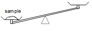
Suppose that you place one, then two, then three 1.0 g calibrated masses into the pan, and that you observe the following:
As a result of these measurements, do you know the mass of the sample? What can you say about the mass of the sample?
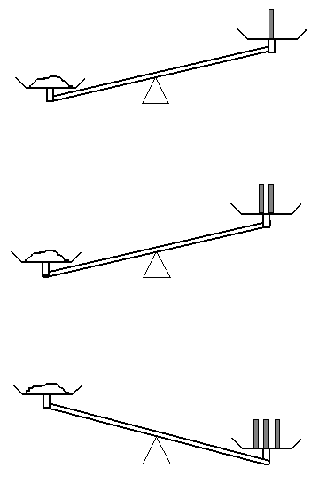
b) Let’s try again. This time, you are provided with 0.2 g calibrated masses as well.
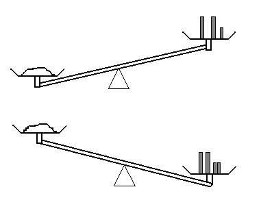
As a result of this measurement, do you know the mass of the sample? What can you say about the mass of the sample this time?
Unless you have a set of more finely calibrated masses lying around (and let me assure you that you do not), you have reached the limit of what this apparatus can tell you about the mass of the sample. This is the origin of the type B evaluation uncertainty. Rather than knowing “the” mass, the measurement gives you an upper and lower bound, hence there is some uncertainty on the measured value.
c) The simplest way to present such a measurement is to provide a single value plus/ minus an uncertainty which covers the entire range of possible values. For example,
1.13 ± 0.04 cm
tells me that the range of a measurement is 1.09 cm to 1.17 cm.
This is standard notation/best form.
In this notation, how would you present the result of part (a) (where you only had 1.0 g masses)?
In this notation, how would you present the results of part (b) (where you had 0.2 g masses)?
Exercise 2
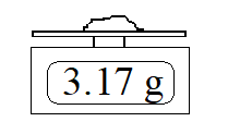
2. You might argue that this type of measurement is crude and lends itself to uncertainty. Why not modernize a bit! Let’s measure a different sample on a (properly calibrated) digital scale …
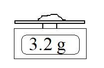 The reading on the scale is clearly 3.2 g, but is the mass of the sample 3.2 g ? The scale only seems capable of giving one decimal place. Could the mass of the sample be 3.18 g? 3.28 g?
How you interpret the scale reading depends on whether the instrument is rounding or truncating.
a) If the instrument is rounding, what are the limits (the highest and lowest possible values) of the measured mass?
What can you say about the mass of the sample? i.e. how would you present the results of this measurement in the standard notation?
b) If the scale is truncating, what are the limits on the measured mass?
What can you say about the mass of the sample? i.e. how would you present the results of this measurement in the standard notation from part 1(c)?
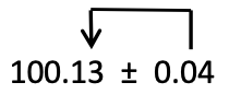
c) What if you were provided with another scale (again properly calibrated) with better precision, as shown here?
 If the instrument is rounding, write an expression for the measurement and uncertainty.
If the instrument is truncating, write an expression for the measurement and uncertainty.
In summary….
There is no such thing as a measurement without uncertainty! No matter how good and how precise your measuring device, there will always be a last decimal place that you can measure, and a next decimal place that you can’t, and so there will always be some limit to what you know about the measured value.
Exercise 3
3. a) The thing you are trying to measure is sometimes called the measurand. In the previous exercise, what was the measurand?
b) An observation:
- When the smallest mass increment you could measure was 1 g (Ex 1a), the uncertainty was 0.5 g.
- When the smallest mass increment was 0.2 g the uncertainty was 0.1 g. (Ex 1b)
- When the smallest increment was 0.01 g the uncertainty was 0.005 g. (Ex 2c).
For these simple scale measurements, summarize the relationship between the uncertainty and the smallest measurement increment.
c) Notice that when a measurement is presented correctly, the precision (i.e. the number of decimal places) of the value matches the precision of the uncertainty:
In this example, you can see that the uncertainty is in the 2nd decimal place, and the last digit of the measurement is the 2nd decimal place. Why does this make sense? (It might be helpful to rephrase the question: what if the precision does NOT match? What if instead of 0.04 as shown, the uncertainty is 4.? 0.4? .004?)
Go back and check the measurements that you wrote down in the previous exercises. Is the precision of every measurement consistent with its uncertainty? If not, how would you correct them?
d) In this introduction to type B uncertainties, we have used the simplest interpretation of the uncertainty – namely that it encompasses the entire range of possible outcomes of the measurement. This is called the maximum uncertainty. For reasons which will only be apparent after we’ve discussed Type A analysis, what is normally presented is called the standard uncertainty which covers approximately 65 % of possible values. Using part 2(a) as an example,
the maximum uncertainty is ± 0.5 g,
the standard uncertainty is ± 0.3 g,
Your final result would be quoted as 1.5 ± 0.3 g.
Go back through your work and rewrite your answers using the standard uncertainty rather than the maximum uncertainty.
Exercise 4
4. a) An analogue instrument, like a ruler or a galvanometer, has a continuous scale.
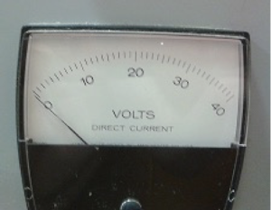
Suppose we want to measure the position of the marker on the diagram below. At a minimum, we would all agree that the marker is over 40 and under 50. From there, you need to use some judgement. What would be your best estimate of the position and its uncertainty? (You might narrow it down this way: what is the measurement definitely NOT? )
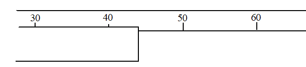
You realize, that procedurally, you are using the same decision-making process as in the digital instrument case to find the uncertainty, i.e. you are asking “what is the possible range of the measurement?”
In principle, its simple! In practice, you can bog down…
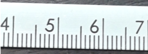
b) Here is a real ruler (in cm) …
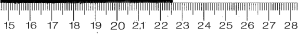
Apply the argument we just made to the marker shown on this scale.
It’s important to be sensible about this so that you don’t waste a lot of time arguing about decimal places that you really can’t measure! We would all agree that the measurement is between 22.50 cm and 22.60 cm. If you decided to use these as the limits of your measurement, what is the maximum uncertainty? How does it compare to the smallest ruled interval?
Now, could you do better, by perhaps getting a magnifying glass and determining whether the marker is in the top half or the bottom half of the interval? Or the top third, the middle third, or the bottom third of the interval? What about the top quarter… bottom quarter? It’s a bit of a slippery slope! The fact is that this ruler is graduated in 10ths, not 100ths. You might reduce the maximum uncertainty from 0.05 to 0.04 or maybe even 0.03, but you aren’t going to change it by a factor of 10. If a measurement hinged on being able to measure that second decimal place precisely, you wouldn’t use this ruler to do the job!
Most importantly!
You need to understand that the process of measuring is entwined with the evaluation of the uncertainty, i.e. you need to assess the uncertainty while making the measurement. This goes for simple measurements (like reading scales) as well as more complicated situations, where external factors limit your ability to measure.
An example of this second case is parallax: if a marker and scale aren’t in the same plane, you can change the apparent position on the scale by moving your head a little bit left or right, up or down. The important thing is to quantify the observation. If you move your head a little bit this way or that way, by how much does it change the measurement? This defines the limits of the measurement, and so the uncertainty. This is not something that you’ll be able to determine once you leave the lab.
(c) Below is a picture of a slit magnified many times. Measure the “width” of the slit with a ruler (the light part in the centre). (If you can print the picture and have a ruler, print and rule. If you have to work from this file, you can use the picture of the ruler (with numbers in cm) and move the vertical line to help with alignment.
Make sure that you provide an estimate of the “Standard uncertainty” (65% of the maximum uncertainty) reported in best form.