Introduction

(Adapted from 1D/1E lab manual, V. Buntar)

From Newton’s Second Law, , the mass of an object determines how effective a certain force will be in producing linear acceleration (i.e. accelerating the object in the direction of the force). In a rotational system, the moment of inertia is the exact analogue of mass in a linear translational system. That is, the moment of inertia, , of an object determines how effective a given torque will be in producing an angular acceleration. The moment of inertia depends not only on the mass of the object but also on how the mass is distributed with respect to the axis of rotation.

The moment of inertia of a point mass can be calculated as

(1)  

where is the mass of the particle and is the distance from the particle to the axis of rotation. If you had a collection of point masses rotating around a single axis then you could calculate the collective moment of inertia by adding up the contribution from each particle with

(2)  

where and are the masses and distances to the axis of rotation for each individual particle, respectively.

Extending to non-idealized objects, that have actual sizes, the treatment gets more complicated because the moment of inertia has a dependence on . How the mass is arranged with respect to the axis of rotation (i.e. the shape) changes the moment of inertia of that object. If you had a lot of time on your hands, it would be possible to split up a real object into point mass particles and then use Equation 2 to calculate the moment of inertia by adding up all the particle inertias.

An example of a simple system is one with two equal point masses equidistant from the axis of rotation. The system you will investigate is slightly more complicated. It consists of a rotating shaft and crossbar on which two disks of total mass are located at a distance from the axis of rotation (see Figure 1). It is designed so that the distance can be easily changed and, hence, the moment of inertia varied. For further details you can watch the first 1.5 minutes of the “How-to” video for this experiment on Avenue to get more familiar with the apparatus.

By measuring both the rotational kinetic energy and the angular velocity of this apparatus, can be determined with respect to the axis of rotation in a dynamical manner. The moment of inertia of the apparatus consists of two parts: there is the moment of inertia of the shaft and crossbar, called , and the moment of inertia of the disk masses placed at a distance , called . Since the moments of inertia simply add (from Equation 2) we can write the total moment of inertia as

(3)  

In this experiment we want to measure , the moment of inertia of the disk masses. To do this, we will measure the moment of inertia of the apparatus with the masses attached,

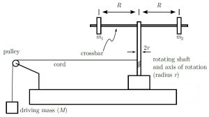
Figure 1: Schematic of crossbar apparatus. Note that the masses m₁ and m₂ are equal and are always placed at equal distances from the rotating shaft.

, and the moment of inertia of the apparatus without the masses, . Then we can simply subtract from to get:

(4)