17.1 Concept and Definition of Reliability
 As discussed in Chapter 4, reliability and consistent performance are critical considerations in the design of new products. Whether a product is repairable (e.g., a stove) or non-repairable (e.g., a light bulb), its total life cycle cost and acquisition cost are significantly influenced by how long it operates without failure, in other words, by its reliability.
Even in service-oriented businesses, operational success depends heavily on the performance of machinery, equipment, and other physical assets. The uninterrupted functioning of these assets is essential, and this can only be ensured through effective maintenance practices.
Reliability and maintenance are, therefore, foundational elements of operations management, directly impacting a firm’s efficiency, service quality, and return on investment. This chapter explores these concepts in detail, supported by numerical examples and practical applications that illustrate their relevance in real-world operational contexts.
Reliability refers to the probability that a machine, product, or system will perform its intended function without failure over a specified period under stated operating conditions. The emphasis on “specified time” is crucial. It reflects the idea of quality sustained over time. In practical terms, when we design, produce, or use products, we expect them to maintain a consistent level of performance throughout their expected lifespan.
Reliability is not limited to individual components; it extends to entire systems. A system typically comprises multiple subsystems, each made up of individual components. The overall reliability of a system depends on the reliability of its constituent parts. In many cases, especially when components are arranged in series, the system’s reliability is the product of the reliabilities of its components. This interdependence highlights the importance of designing and maintaining each part to ensure the system functions as intended.
Reliability is a key performance metric in both manufacturing and service operations, influencing product quality, customer satisfaction, and operational efficiency.
System Reliability
In operations management and engineering design, system reliability refers to the likelihood that an entire system will function without failure over a specified period. For a system composed of n components arranged in series, the system reliability is calculated as the product of the reliabilities of each individual component:
Rs = R1 x R2 x… x Rn
Example
Consider a system with four components arranged in series, where:
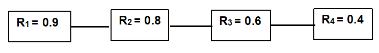
Where R1 = 0.9, R2 = 0.8, R3 = 0.6, R4 = 0.4
The system reliability is: RS = 0.9 × 0.8 × 0.6 × 0.4 = 0.1728
This means the system has a 17.28% chance of functioning without failure over the specified time period.
It is important to note that although each individual component has a relatively high reliability, the overall system reliability is significantly lower. This is because in a series configuration, the system fails if any one component fails. As more components are added in series, the probability of system failure increases, resulting in a decline in overall reliability.
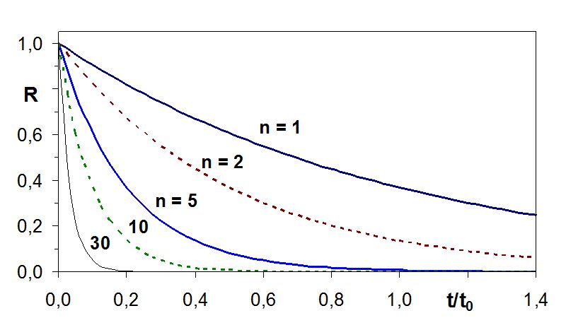
Figure 17.1.2 illustrates how system reliability decreases as the number of components in series increases.
17.1.2 Image Description
A line graph shows the reliability function 𝑅 (vertical axis, ranging from 0 to 1) versus normalized time 𝑡/𝑡0 (horizontal axis, ranging from 0.0 to 1.4). Multiple curves are plotted for different values of 𝑛. The curve for
𝑛=1(blue solid line) decreases steadily and more slowly compared to the others. The curve for 𝑛=2(red dashed line) declines faster than𝑛=1. The 𝑛=5 curve (blue solid line) drops more steeply. The curves for 𝑛=10 (green dashed line) and 𝑛=30 (thin black line) decline sharply near the beginning and approach zero quickly. Labels “n = 1,” “n = 2,” “n = 5,” “10,” and “30” are placed near their respective curves. The graph illustrates that reliability decreases faster with increasing values of 𝑛.
To counteract this decline, designers often introduce redundancy, meaning additional components or backup systems that can take over in case of failure. Redundancy can significantly improve system reliability, especially in critical applications.
Redundancy in System Reliability
Redundancy refers to the inclusion of additional or backup components in a system to enhance its overall reliability. In a redundant system, components are arranged in parallel, meaning the system continues to function as long as at least one of the parallel components is operational. The system only fails when all redundant components fail.
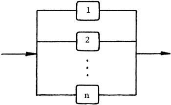
Redundancy can involve one or more backup units. For example, an n-unit parallel system includes multiple components operating in parallel, any of which can sustain the system’s functionality.
17.1.3 Image Description
A schematic diagram showing a parallel system with 𝑛 components. Each component, labelled 1, 2, …, n, is represented by a rectangular block connected between two horizontal lines. The left arrow indicates system input, and the right arrow indicates system output. The diagram illustrates that the system continues to operate as long as at least one component functions, representing a parallel reliability configuration.
The reliability of such systems is often calculated using the complement of unreliability, expressed as:

Where:
- Rsys is the system reliability,
- R(t) is the reliability of a single component over time t,
- n is the number of parallel components.
This formula is derived using the Cumulative Distribution Function (CDF), which represents the probability of failure up to a given point in time.
Example: Two-Unit Parallel System
Consider a system with two identical pumps, each with a reliability of 0.7. The system will function as long as at least one pump is operational. The reliability of the system is calculated as:
Rs = R1 + (R2)( 1- R1)
Illustrating the above formula in more detail,
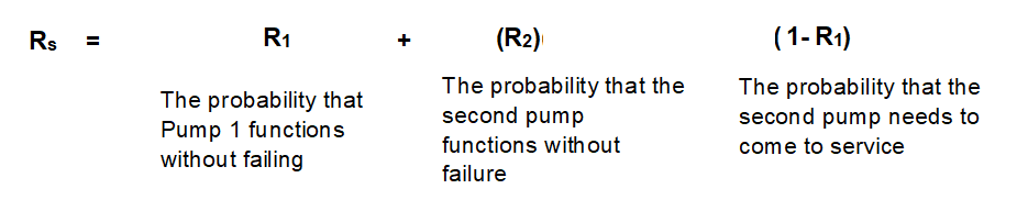
R1: The probability that Pump 1 functions without failing.
𝑅2: The probability that the second pump functions without failure.
(1−𝑅1): The probability that the second pump needs to come into service.
The formula represents how the total system reliability 𝑅𝑠 depends on the reliability of each pump in a parallel configuration.
Rs = R1 + (R2)( 1- R1)
Rs = 0.7 + 0.7(1−0.7) = 0.7 + 0.21 = 0.91
Thus, the dual-pump system has a 91% chance of operating without failure, significantly higher than the reliability of a single pump.
Example: Redundancy in a Four-Component System
Let’s revisit the earlier four-component series system:
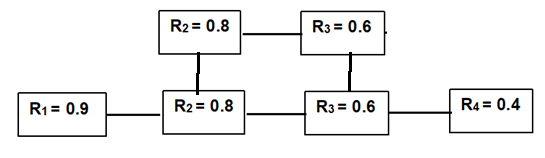
Without redundancy, the system reliability was:
Rs = 0.9 × 0.8 × 0.6 × 0.4 = 0.1728 or 17.28%
Now, suppose R₂ and R₃ are each backed up by identical components (i.e., parallel redundancy). The new system reliability becomes:
Rs = R1 × [R2 + R2 (1−R2)] × [R3 + R3 (1−R3)] × R4
Substituting the values:
Rs = 0.9 × [0.8 + 0.8 (1−0.8)] × [0.6 + 0.6 (1−0.6)] × 0.4 = 0.9 × 0.96 × 0.84 × 0.4 = 0.2903 or 29.03%
This demonstrates a significant improvement in system reliability—from 17.28% to 29.03%—achieved by introducing redundancy in just two components (Schenkelberg, n.d.).
Interdependence in System Reliability
Interdependence refers to the relationships and dependencies among components or subsystems within a larger system. In interdependent systems, the failure of one component can trigger cascading failures in others, increasing the system’s vulnerability. This phenomenon is particularly evident in complex systems such as weather models, financial markets, or power grids, where changes follow stochastic patterns and are often modelled using advanced tools like Markov Chains. While such modelling is beyond the scope of this textbook, the concept of interdependence remains central to understanding system reliability.
Incorporating redundancy into interdependent networks can mitigate the impact of cascading failures by providing alternative pathways or backup components, thereby enhancing overall system resilience.
In less complex systems, interdependence can be analyzed by examining how failures propagate through a process chain, affecting the final yield or performance. The following scenarios illustrate how interdependence influences reliability and how recovery mechanisms can improve outcomes.
Scenario 1: Interdependent Production Stages
Consider a production line with two consecutive stages:
- Stage 1 Reliability: 90%
- Stage 2 Reliability: 90% (if operating independently)
However, if Stage 1 fails, Stage 2 has only a 40% chance of success due to its dependency on Stage 1’s output.
Independent Case (No Interdependence)
- Rsind=0.9×0.9=0.81
Interdependent Case
Let’s break down the probabilities:
- Both stages succeed:
0.9 × 0.9 = 0.81 - Stage 1 succeeds, Stage 2 fails:
0.9 × 0.1 = 0.09 - Stage 1 fails, Stage 2 succeeds (via rework):
0.1 × 0.4 = 0.04 - Both stages fail:
0.1 × 0.6 = 0.06
Total System Reliability (Interdependent)
Rs=0.81+0.04=0.85
This example shows that recovery mechanisms, such as rework or redundancy, can improve reliability even in interdependent systems. However, interdependence generally introduces complexity and potential fragility compared to fully independent systems.
Scenario 2: Wastewater Treatment Filter
In a wastewater treatment plant, a specialized filter is used to remove pathogens during peak flow hours. The system has the following characteristics:
- Initial success rate: 90%
- Usability after peak flow: 80%
- Retrofit success rate: 50% of usable filters
- Fallback success rate: 33% of non-retrofitted filters

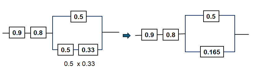
17.1.7 Image Description
A labelled reliability block diagram showing two series components (0.9 and 0.8) followed by two parallel paths: one with a single block labelled 0.5, and the other with two series blocks labelled 0.5 and 0.33. Blue text annotations explain the meaning of each value: “90% success removing pathogen” beside 0.9, “80% remain usable after contact” beside 0.8, “Half (50%) can be retrofitted to be usable” beside the top 0.5, “Half (50%) cannot be retrofitted” beside the lower 0.5, and “A third (33%) can be used” beside 0.33. The diagram visually represents a system reliability scenario related to usable and non-usable components after processing.
To determine the overall reliability, we analyze the network of dependencies:
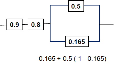
17.1.8 Image Description
Two reliability block diagrams are shown side by side. On the left, two components labelled 0.9 and 0.8 are in series, followed by two parallel branches: one with a single block labelled 0.5 and another with two series blocks labelled 0.5 and 0.33. Below the diagram, the formula “0.5 × 0.33” appears. An arrow points to the simplified right-hand diagram, which shows the 0.9 and 0.8 series components followed by parallel blocks labelled 0.5 and 0.165, representing the equivalent system reliability simplification.
As shown below, the yield of the parallel components can be calculated.
17.1.9 Image Description
A reliability block diagram with two components in series, labelled 0.9 and 0.8, followed by two components in parallel, labelled 0.5 and 0.165. Below, a formula shows: “0.165 + 0.5(1 − 0.165).”
And with that calculation, three serial components exist whose collective yield is easily calculated as shown below.
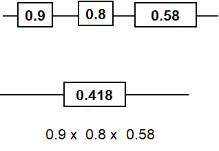
17.1.10 Image Description
A reliability block diagram showing three components connected in series, each labelled with reliabilities of 0.9, 0.8, and 0.58. Below the diagram, there is a single block labelled 0.418, with a formula underneath: “0.9 × 0.8 × 0.58.”
Therefore, based on the above-mentioned interdependencies, this filter has a success probability of 41.8% to remove the pathogens in an hour of peak flow (Rahnamay-Naeini, 2016).
“Basic Terms of Reliability” & “Reliability of Systems” from Concise Reliability for Engineers by Jaroslav Mencik is licensed under a Creative Commons Attribution 3.0 License,
