14.5 Mathematical Approaches to Aggregate Planning
Mathematical models provide a structured and quantitative foundation for aggregate planning, enabling decision-makers to optimize resource allocation while meeting demand constraints. Two widely used methods are Linear Programming (LP) and the Transportation Model.
Linear Programming
Linear programming is a powerful optimization technique used to minimize total production costs while satisfying demand and capacity constraints. Consider the following example:
Example
Problem Context
A company produces two special-order products, A and B, with unit production costs of $50 and $70, respectively. Due to commitments to other products, the company has limited production capacity for special orders over the next three months:
| Month | Available Capacity (units) |
|---|---|
| 1 | 100 |
| 2 | 120 |
| 3 | 110 |
Projected demand for products A and B is:
| Month | Demand A | Demand B |
|---|---|---|
| 1 | 20 | 20 |
| 2 | 40 | 30 |
| 3 | 50 | 40 |
Formulation
Let:
- x1, x2, x3: Units of Product A produced in Months 1, 2, and 3
- y1, y2, y3: Units of Product B produced in Months 1, 2, and 3
Objective Function:
Minimize total cost:
Z = 50(x1 + x2 + x3) + 70(y1 + y2 + y3)
Subject to Constraints.
Capacity Constraints:
- x1 + y1 ≤ 100
- x2 + y2 ≤ 120
- x3 + y3 ≤ 110
Demand Constraints:
- x1 ≥ 20, x2 ≥ 40, x3 ≥ 50
- y1 ≥ 20, y2 ≥ 30, y3 ≥ 40
Non-negativity:
- xi, yi ≥ 0 for all i
This problem can be solved using the Simplex Method or other LP solvers, as discussed in Chapter 16.
Farnsworth Transportation Model
The transportation model is particularly useful when demand can be met through multiple sources, such as regular production, overtime, subcontracting, and inventory carryover. It aims to minimize total cost while satisfying demand across multiple periods.
Example
Problem Context
A hardwood flooring manufacturer must meet the following monthly demand for solid oak flooring:
| Month | Demand (m2) |
|---|---|
| 1 | 5,000 |
| 2 | 15,000 |
| 3 | 20,000 |
| 4 | 5,200 |
Available Resources and Costs:
- Beginning Inventory: 500 m²
- Regular Production: 5,000 m²/month at $40/m²
- Overtime Capacity: 5,000 m²/month at $75/m²
- Subcontracting: 4,000 m²/month at $85/m²
- Inventory Holding Cost: $2/m²/month
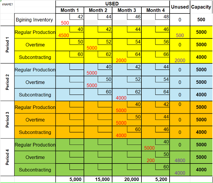
The three measures available to the company are regular production, using overtime, and subcontracting. Within the context of the transportation model, we can assume that these measures are the sources of supply for which we have four market demands, as shown in the following table.
Approach
The goal is to allocate production and inventory resources across four months to minimize total cost. The steps include:
- Utilize Beginning Inventory: Use the 500 m² from the previous month to avoid holding costs.
- Prioritize Low-Cost Options: Use regular production first, followed by overtime and subcontracting.
- Carry Over Excess Capacity: If demand is unmet in a given month, use surplus from previous months.
Monthly Breakdown
- Month 1:
- 500 m² from inventory
- 4,500 m² from regular production
- Total: 5,000 m² (demand met)
- Month 2:
- 5,000 m² from regular production
- 5,000 m² from Month 1 overtime (carried forward)
- 5,000 m² from overtime
- Total: 15,000 m² (demand met)
- Month 3:
- 5,000 m² from regular production
- 5,000 m² from overtime
- 4,000 m² from subcontracting
- 6,000 m² from subcontracting carried out in previous months
- Total: 20,000 m² (demand met)
- Month 4:
- 5,000 m² from regular production
- 200 m² from overtime
- Total: 5,200 m² (demand met)
Cost Calculation
By summarizing the quantities used from each source and applying the respective costs, the total cost of the four-month plan is:
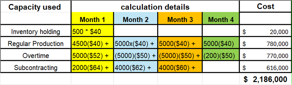
Image Description
| Capacity used | Calculation details | Cost | |||
|---|---|---|---|---|---|
| Month 1 | Month 2 | Month 3 | Month 4 | ||
| Inventory holding | 500 * $40 | $20,000 | |||
| Regular Production | 4500($40) + | 5000($40) + | 5000($40) + | 5000($40) | $780,000 |
| Overtime | 5000($52) + | 5000($50) + | 200($50) | $770,000 | |
| Subcontracting | 2000($64) + | 4000($62) + | 4000($60) + | $616,000 | |
| $2,186,000 | |||||
Total Cost: $2,186,000
This solution meets all demand requirements while minimizing costs through optimal use of available resources.
