12.5 Solving a Transportation Problem Using the Simplex Method in Excel Solver
In Chapter 11, we solved a transportation problem using the Stepping Stone and MODI methods. We will now revisit the same problem and solve it using the Simplex Method via Excel Solver.
Initial Transportation Cost
Using the initial basic feasible solution, the firm’s transportation cost is calculated as follows:
| M1 | M2 | M3 | ||
|---|---|---|---|---|
| DC1 | 150 6 | 50 9 | 16 | 0 |
| DC2 | 11 | 150 10 | 50 7 | 0 |
| DC3 | 16 | 12 | 200 10 | 0 |
| 0 | 0 | 0 |
Total Cost:
150(6) + 50(9) + 150(10) + 50(7) + 200(10) = $5,200
Stepping Stone Method
Using the Stepping Stone Method, the optimal solution was found to be:
150(6) + 50(9) + 0(10) + 200(7) + 150(12) + 50(10) = $5,050
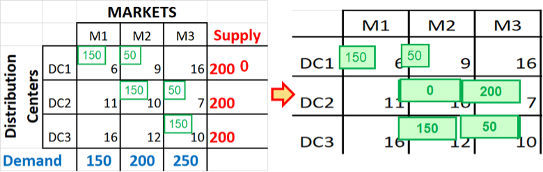
12.5.2 Image Description
Two side-by-side transportation tables for a supply and demand allocation problem.
Left table: Distribution centers (DC1, DC2, DC3) are listed on the left, markets (M1, M2, M3) along the top. Each cell shows a shipping cost, with green numbers indicating allocated units. Supply is listed in red on the right (200 for each DC, with DC1 showing 0 remaining), and demand in blue along the bottom (150 for M1, 200 for M2, 250 for M3). Allocations: DC1 sends 150 to M1 and 50 to M2; DC2 sends 150 to M2 and 50 to M3; DC3 sends 150 to M1 and 50 to M3.
Right table: The same allocations are redrawn with green boxes around the numbers, visually emphasizing how shipments from DCs are distributed to meet the demands of markets.
Linear Programming Method
We will now formulate this problem as a linear programming problem (LPP) and solve it using the Excel Solver.
Objective: Minimize total transportation cost:
| MARKETS | |||||
| M1 | M2 | M3 | Supply | ||
| Distribution Centers | DC1 | X11
6 |
X12
9 |
X13
16 |
200 |
| DC2 | X21
11 |
X22
10 |
X23
7 |
200 | |
| DC3 | X31
16 |
X32
12 |
X33
10 |
200 | |
| Demand | 150 | 200 | 250 | ||
Minimize Z
[latex]Z:\; \min TC = \begin{aligned} &X_{11}(6) + X_{12}(9) + X_{13}(16) \\ &+ X_{21}(11) + X_{22}(10) + X_{23}(7) \\ &+ X_{31}(16) + X_{32}(12) + X_{33}(10) \end{aligned}[/latex]
Subject to supply constraints:
- X11+X12+X13 ≤ 200
- X21+X22+X23 ≤ 200
- X31+X32+X33 ≤ 200
And demand constraints:
- X11+X21+X31 ≤ 150
- X12+X22+X32 ≤ 200
- X13+X23+X33 ≤ 250
All decision variables Xij ≥ 0
Implementing in Excel
- Set up the cost matrix and decision variables in Excel.
- Use SUMPRODUCT formulas to compute the total cost and the left-hand sides of the constraints.
- Verify that all formulas are correctly implemented.
- Open Solver and configure:
- Objective: Minimize the total cost of the cell.
- Variable Cells: All Xij decision variables.
- Constraints: Supply and demand constraints as listed above.
- Solving Method: Select Simplex LP.
| X11 | X12 | X13 | X21 | X22 | X23 | X31 | X32 | X33 | Left | Right | |
| OBJE | 6 | 9 | 16 | 11 | 10 | 7 | 16 | 12 | 10 | ||
| D1 | 1 | 11 | 200 | ||||||||
| D2 | 1 | 1 | 1 | 200 | |||||||
| D3 | 1 | 1 | 1 | 200 | |||||||
| M1 | 1 | 1 | 1 | 150 | |||||||
| M2 | 1 | 1 | 1 | 200 | |||||||
| M3 | 1 | 1 | 1 | 250 | |||||||
| SOLUTION | 0 | 0 | 0 | 0 | 0 | 0 | 0 | 0 | 0 |
After all SUMPRODUCT formulas have been correctly implemented and verified, the model is now fully prepared for optimization. The Solver-ready layout of the transportation problem is shown below:
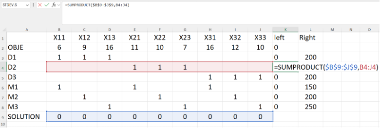
12.5.5 Image Description
An Excel spreadsheet showing a linear programming or optimization setup with decision variables, constraints, and an objective function. The columns labelled X11 through X33 represent variables, while rows D1 to D3 and M1 to M3 list constraints. Row 2 (D1) has ones under X11, X12, and X13. Row 3 (D2) has ones under X21, X22, and X23. Row 4 (D3) has ones under X31, X32, and X33. Additional rows M1 to M3 contain other combinations of ones under different variables. The "OBJE" row at the top lists objective coefficients such as 6, 9, 16, 11, 10, etc. Columns K (“left”) and L (“Right”) contain constraint results, with right-hand side values 200, 150, 200, and 250. Row 10 ("SOLUTION") currently has zeros under all variables. A formula bar shows =SUMPRODUCT($B$9:$J$9,B4:J4)
The optimized solution, as computed by Excel Solver, is presented below:
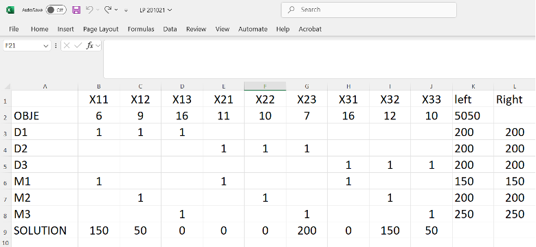
12.5.6 Image Description
An Excel spreadsheet illustrating a linear programming solution, featuring variables X11–X33, objective values, demand and supply constraints, and solution values. The final solution assigns nonzero values to X11, X12, X23, X32, and X33, achieving an objective total of 5050.
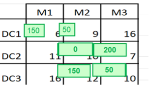
12.5.7 Image Description
A transportation table showing supply nodes (M1, M2, M3) across the top and demand centers (DC1, DC2, DC3) along the side. Each cell contains a cost value, with green boxes displaying allocated shipment quantities. Allocations are: 150 from M1 to DC1, 50 from M2 to DC1, 200 from M2 to DC2, 150 from M1 to DC3, and 50 from M2 to DC3. Other routes have no allocation.
Solver Output
After solving, Excel Solver returns the following optimal allocation:
[latex]150(6) + 50(9) + 0(10) + 200(7) + 150(12) + 50(10) = 5{,}050[/latex]
This matches the optimal solution previously obtained using the Stepping Stone method, confirming the validity of the Simplex-based approach in Excel.
