12.4 Solving a Linear Programming Problem (LPP) Using Excel Solver
In addition to the Simplex Method, the Linear Programming Problem (LPP) can also be solved using Excel Solver, a powerful optimization tool available in Microsoft Excel. Below, we outline the step-by-step process for formulating and solving the LPP in Excel.
Step 1: Formulate the LPP in Excel
Consider the following LPP:
| Biscuit ([latex]x_{1}[/latex]) | Cupcakes ([latex]x_{2}[/latex]) | ||
|---|---|---|---|
| Objective | 5 | 4 | [latex]Z[/latex] |
| Mixer | 3 | 5 | 78 |
| Oven | 4 | 1 | 36 |
| Solution ([latex]x_{1}, x_{2}[/latex]) | 0 | 0 |
Step 2: Define the Objective Function
Initially, we enter 0 for both decision variables ([latex]x_{1}[/latex] and [latex]x_{2}[/latex]) in the solution row. The objective function is defined using the SUMPRODUCT function in Excel:
12.4.2 Image Description
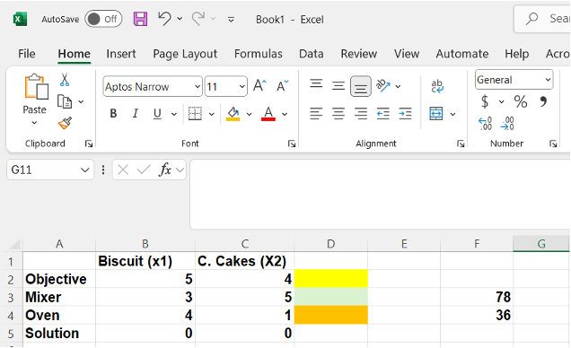
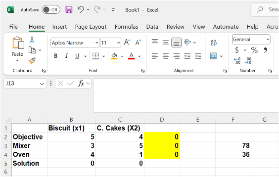
A Microsoft Excel spreadsheet displays a table used for linear programming or resource allocation, comparing the production of Biscuits (x1) and Cakes (x2). The table includes rows labelled "Objective," "Mixer," "Oven," and "Solution."
- The "Objective" row lists the profit per unit: 5 for Biscuits and 4 for Cakes.
- The "Mixer" row shows the resource requirements: 3 for Biscuits and 5 for Cakes, with a constraint of 78 (in cell F2).
- The "Oven" row shows requirements: 4 for Biscuits and 1 for Cakes, with a constraint of 36 (in cell F3).
- The "Solution" row currently contains zeros for both products.
Coloured cells highlight different resource rows, likely for visual differentiation purposes. Columns are labelled from B to F.
Once the solution is obtained, the initial zero values assigned to the decision variables [latex]x_{1}[/latex] and [latex]x_{2}[/latex] will be replaced by non-negative optimal values. It is important to understand that these variables serve as coefficients in the SUMPRODUCT function, which calculates the objective function and the left-hand sides of the constraints.
To enable Excel Solver to process the LPP correctly, the relationship between the decision variables and the objective function must be explicitly defined. This is done by entering a SUMPRODUCT formula in the objective cell (e.g., cell D2), which multiplies the values of [latex]x_{1}[/latex] and [latex]x_{2}[/latex] (from the solution range) by their corresponding objective coefficients.
For example, the formula might look like this:
12.4.3 Image Description
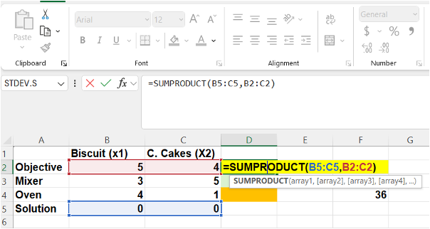
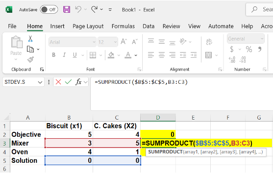
A Microsoft Excel spreadsheet shows a formula being entered in cell D5: =SUMPRODUCT(B5:C5,B2:C2). The table compares two products: Biscuits (x1) and Cakes (x2), with rows for "Objective," "Mixer," "Oven," and "Solution." The formula highlights the "Solution" row (B5:C5) and the "Objective" row (B2:C2), indicating a dot product to calculate total profit. The calculated result, 36, appears in cell G4 (corresponding to the Oven constraint). The formula bar and syntax helper are also visible, and cells are colour-coded for clarity: red for the "Objective" row, blue for the "Solution" row, and yellow for the formula cell.
In this formula:
- The blue-highlighted cell references (e.g., $B$5:$C$5) represent the solution range (i.e., the decision variables).
- The red-highlighted cell references (e.g., B2:C2) represent the objective function coefficients.
The use of absolute references (with dollar signs) ensures that the solution range remains fixed when the formula is copied to other cells, such as those used to compute the constraint expressions.
12.4.4 Image Description
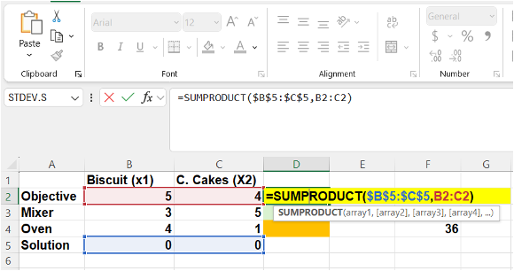
An Excel spreadsheet shows the formula =SUMPRODUCT($B$5:$C$5,B2:C2) entered in cell D2, highlighted in yellow. The formula multiplies the values in the "Solution" row (row 5, cells B5 and C5, shown in blue) with the "Objective" coefficients (row 2, cells B2 and C2, shown in red) to calculate a total value. The dollar signs in $B$5:$C$5 indicate absolute references. The SUMPRODUCT function is displayed in the formula bar with its syntax hint below. The table tracks inputs for Biscuits (x1) and Cakes (x2) and includes rows for Objective, Mixer, Oven, and Solution. The result "36" is displayed in cell G4.
After entering the formula, press Enter. At this stage, the Linear Programming Problem (LPP) in Excel will reflect the initial setup. The value displayed in the objective cell (e.g., cell D2) will be zero. This result is expected, as it represents the SUMPRODUCT of the initial decision variable values (both set to zero) and their corresponding objective function coefficients (5 and 4). Since any number multiplied by zero yields zero, the objective function currently evaluates to zero.
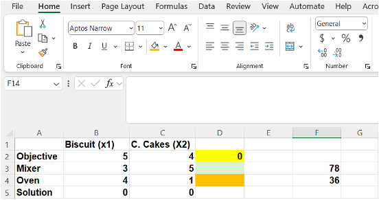
Figure 12.4.5 Image Description
An Excel spreadsheet displays a linear programming-style table used for resource allocation between two products: Biscuits (x1) and Cakes (x2). The rows include "Objective," "Mixer," "Oven," and "Solution."
- The "Objective" row shows the profit per unit: 5 for Biscuits and 4 for Cakes.
- The "Mixer" and "Oven" rows show the resource requirements for each product, with constraints of 78 and 36 listed in column F.
- The "Solution" row has zeros for both products (x1 = 0, x2 = 0).
- Cell D2 is highlighted yellow and contains the value 0, representing the calculated total objective value based on the solution (likely using the SUMPRODUCT function).
- Some cells in the "Mixer" and "Oven" rows are highlighted in gradient colours for visual emphasis.
Next, the formula entered in the objective cell (e.g., the yellow cell) should be copied to the cells corresponding to the constraint rows (e.g., the green and orange cells). This ensures that the left-hand side of each constraint is also calculated using the SUMPRODUCT of the decision variables and the respective constraint coefficients.
To do this, click on the bottom-right corner of the yellow cell (which contains the SUMPRODUCT formula) and drag it downward to cover the constraint rows. Since the current values of [latex]x_{1}[/latex] and [latex]x_{2}[/latex] are both zero, the resulting calculations in the constraint cells will also be zero. This is expected, as multiplying zero-valued decision variables by any coefficients yields zero.
This step confirms that the formulas are correctly replicated and that the structure of the model is consistent across the objective and constraint rows.
12.4.6 Image Description
An Excel spreadsheet displays a resource allocation table for two products: Biscuits (x1) and Cakes (x2). The table includes rows labelled "Objective," "Mixer," "Oven," and "Solution."
- The "Objective" row shows profit per unit: 5 for Biscuits and 4 for Cakes.
- The "Mixer" row lists resource usage: 3 for Biscuits and 5 for Cakes, with a constraint of 78 in cell F3.
- The "Oven" row lists resource usage: 4 for Biscuits and 1 for Cakes, with a constraint of 36 in cell F4.
- The "Solution" row contains 0 units for both Biscuits and Cakes.
- Column D contains calculated values for each row, all currently 0 and filled with a yellow background, suggesting these are formula outputs (e.g.,
SUMPRODUCTcalculations). - The interface includes the Excel ribbon and a blank formula bar, with no formula currently selected.
To verify that the formulas have been correctly copied into the constraint rows, you can double-click on any of the corresponding cells. Doing so will highlight the cell references involved in the formula, allowing you to visually confirm that the correct rows and columns are being used in the SUMPRODUCT calculation.
12.4.7 Image Description
An Excel spreadsheet shows a calculation using the SUMPRODUCT function in cell D3, highlighted in yellow. The formula is =SUMPRODUCT($B$5:$C$5,B3:C3), which multiplies values from the "Solution" row (row 5, shown in blue) with the corresponding values from the "Mixer" row (row 3, shown in red) for Biscuits (x1) and Cakes (x2). The result, currently 0, is displayed in cell D3. The table includes rows for Objective, Mixer, Oven, and Solution, and columns for product types. Resource constraints are listed in column F (78 for Mixer and 36 for Oven). The formula bar is visible at the top, with SUMPRODUCT syntax help displayed.
With all SUMPRODUCT formulas correctly defined and verified, the model is now ready to be solved using Excel Solver.
To access Solver, follow these steps:
- Click on the Data tab located at the top of the Excel window.
- In the Data ribbon, locate and click on Solver, typically found on the far right.[1]
- The Solver Parameters dialogue box will appear. For convenience, you may drag this dialogue box closer to your LPP model on the worksheet.
Click through the following to see the steps:
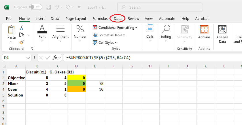


Image Description
Image 1: An Excel spreadsheet is open with a pop-up instruction pointing to the "Data" tab in the ribbon, which is circled in red. The instruction reads: "Click on the Data tab located at the top of the Excel window."
Image 2: An Excel spreadsheet is open with a highlighted instruction pointing to the "Solver" tool in the "Data" ribbon. A red circle emphasizes the "Solver" button on the far right of the ribbon. A text box says: “In the Data ribbon, locate and click on Solver, typically found on the far right.”.
Image 3: An Excel spreadsheet is open with the "Solver Parameters" dialogue box displayed in the foreground. The dialogue box includes fields for setting the objective cell, selecting Max or Min, and specifying changing variable cells and constraints. A note on the spreadsheet reads: “The Solver Parameters dialogue box will appear. For convenience, you may drag this dialogue box closer to your LPP model.”
At this stage, the Solver Parameters dialogue box prompts you to input the necessary model components. Essentially, Solver requires you to define the objective function, specify the decision variables, and set the constraints that govern the Linear Programming Problem (LPP).
Click through to see the steps:
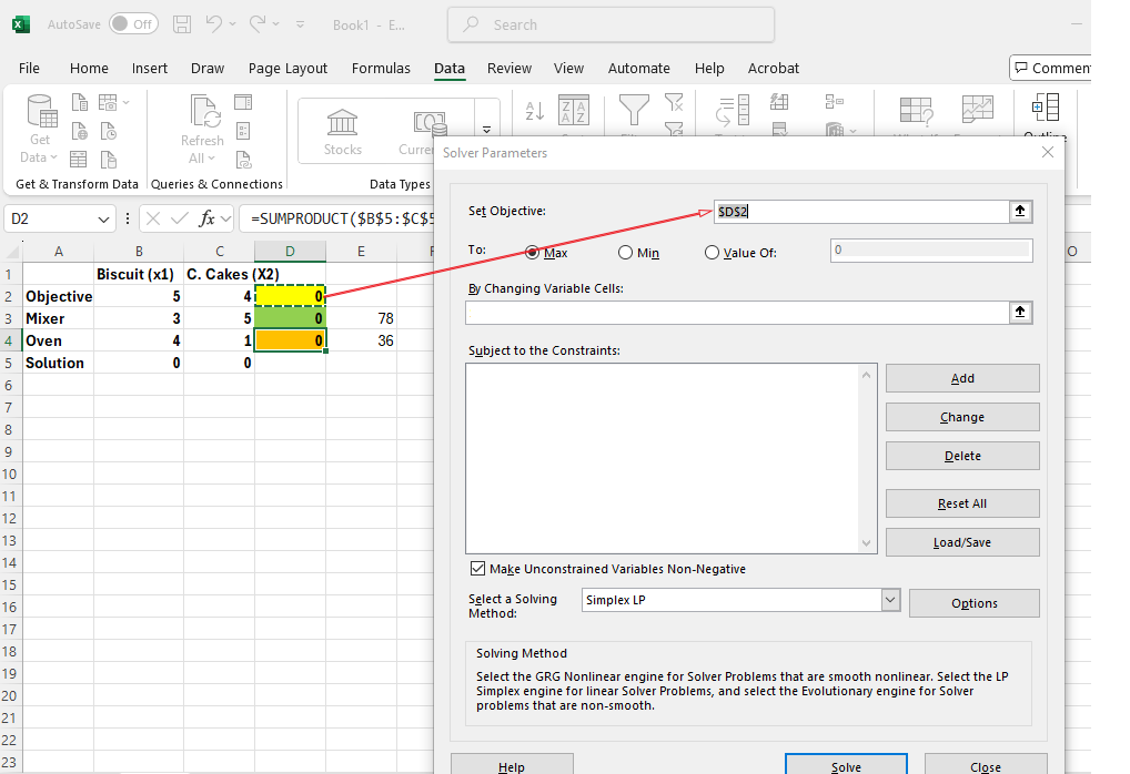
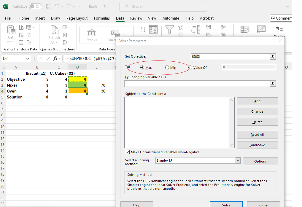
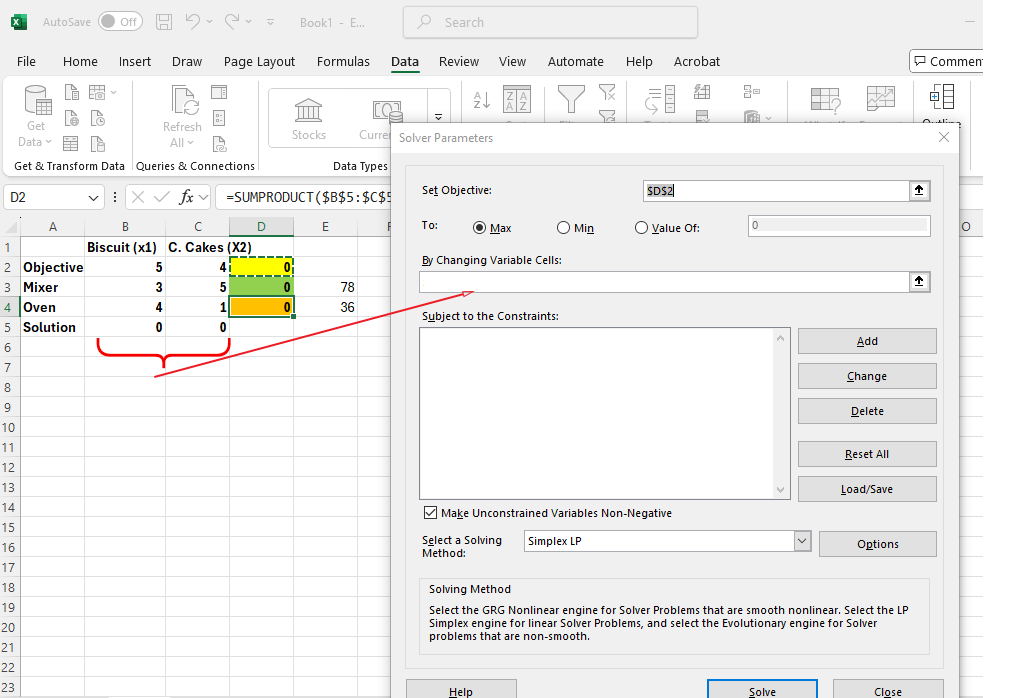
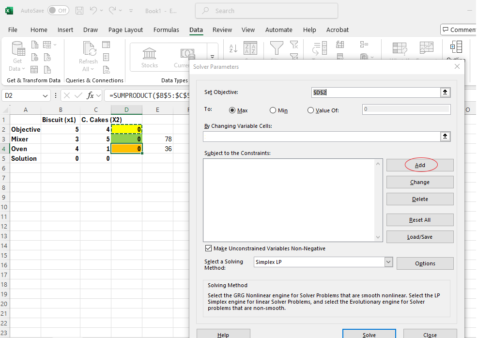
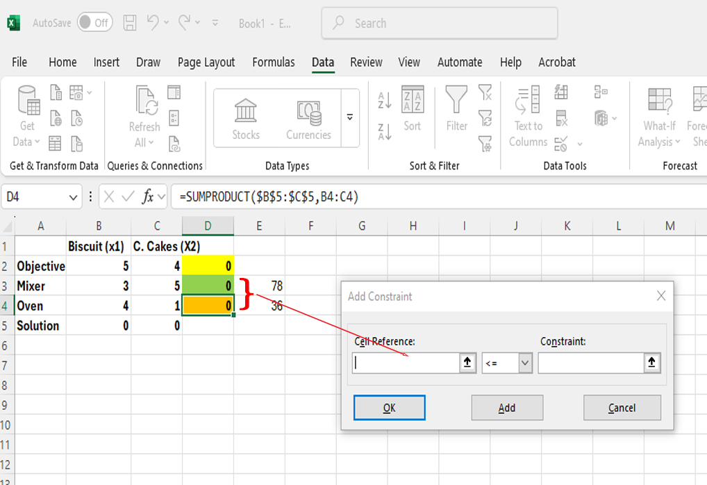
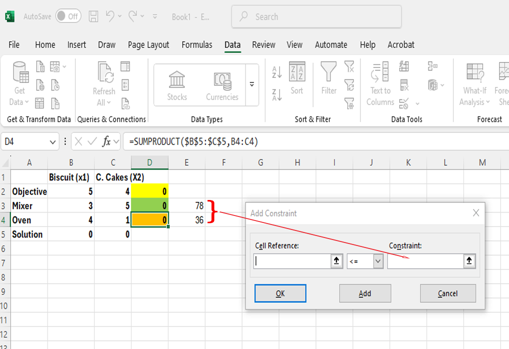
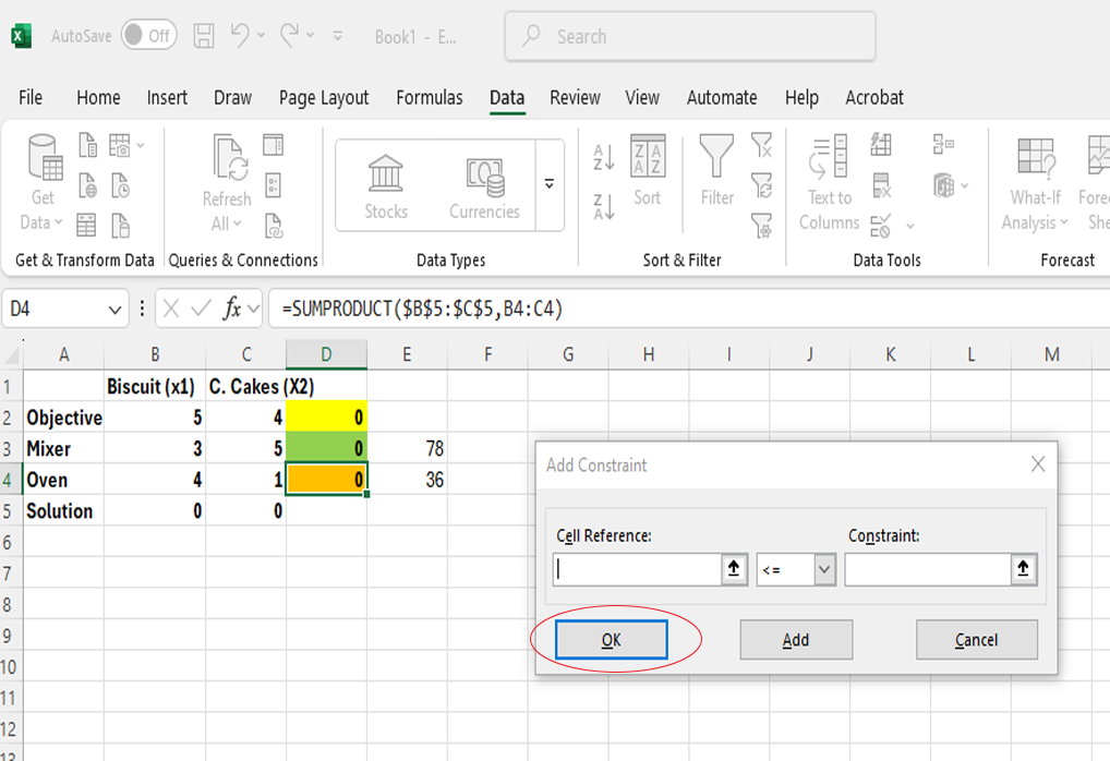
Image Description
Image 1: An Excel spreadsheet is shown with the "Solver Parameters" dialogue box open in the foreground. A red arrow points from the "Set Objective" field in the dialogue box to cell D2 in the spreadsheet, which is highlighted in green. A callout reads: “Step 1: Enter this cell.” The Solver dialogue box is used for setting up an optimization model. The spreadsheet in the background includes a linear programming problem with rows for Objective, Mixer, Oven, and Solution, and columns for two products: Biscuits (x1) and Cakes (x2). Calculated values in column D are highlighted in yellow, and resource limits appear in column E (78 for Mixer and 36 for Oven).
Image 2: An Excel spreadsheet with the "Solver Parameters" dialogue box open in the foreground. A callout labelled “Step 2: Max? or Min?” points to the "Set Objective" section of the dialogue box, where options to select either "Max" (maximize) or "Min" (minimize) are shown, with "Max" currently selected.
Image 3: An Excel spreadsheet is open with the "Solver Parameters" dialogue box displayed in the foreground. A red arrow points from the "Subject to the Constraints" section in the Solver box to the solution cells B5 and C5 in the spreadsheet, which contain zeros. A callout labelled “Step 3: Select the solution range and enter” is shown beside the constraint entry area.
Image 4: An Excel spreadsheet with the "Solver Parameters" dialogue box open in the foreground. A callout labelled “Step 4: Add the constraint by clicking on the Add Button” points to the "Add" button on the right side of the dialogue box, which is circled in red. The dialogue box includes options to set the objective, select Max or Min, and define changing variable cells and constraints.
Image 5: An Excel spreadsheet with the "Add Constraint" dialogue box open in the foreground. A red arrow points from the "Cell Reference" field in the dialogue box to cells D3 and D4 in the spreadsheet, which contain the values 0 and are highlighted in green and yellow. A callout labelled “Step 5: Select the left constraint range and enter” explains this action.
Image 6: An Excel spreadsheet is open with the "Add Constraint" dialogue box in the foreground. A red arrow points from the "Constraint" field in the dialogue box to cells G3 and G4 in the spreadsheet, which contain the values 78 and 36, representing resource limits for Mixer and Oven, respectively. A callout labelled “Step 6: Select the right constraint range and enter” explains this step.
Image 7: An Excel spreadsheet with the "Add Constraint" dialogue box open in the foreground. A callout labelled “Step 7: Click OK” points to the OK button, which is circled in red. The dialogue box contains filled-in fields for “Cell Reference” and “Constraint,” referring to the left (D3:D4) and right (E3:E4) constraint ranges in the spreadsheet.
Once the required parameters have been entered, the Solver Parameters dialogue box will be fully populated and ready for review, as illustrated below:
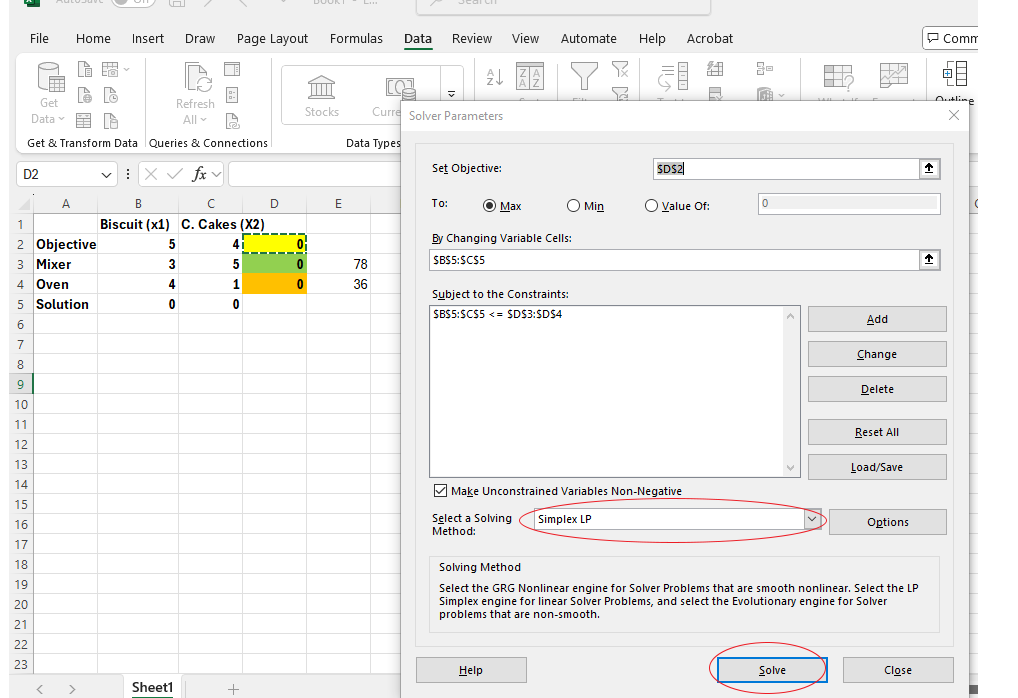
12.4.8 Image Description
Final Steps in Using Excel Solver
To complete the optimization process, follow these final steps:
- Select the Solving Method:
In the Solver Parameters dialogue box, choose Simplex LP from the Select a Solving Method dropdown menu. This method is appropriate for linear programming problems. - Click Solve:
Once all parameters are correctly set, click the Solve button. Solver will process the model and return the optimal solution. - Review and Accept the Solution:
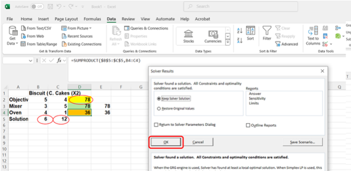
After Solver finds a solution, a dialogue box will appear displaying the results. Click OK to accept the solution and close the dialogue box. The optimal values will now be reflected directly in the Excel worksheet.
Interpreting the Solution
- Decision Variables (Solution Row):
Solver indicates that to maximize the objective function, the optimal solution is:- [latex]x_{1}[/latex] (Biscuits) = 6 units
- [latex]x_{1}[/latex] (Cupcakes) = 12 units
- Objective Function:
The maximum profit (objective value) is [latex]\$78[/latex]. - Constraints:
- The Mixer constraint is fully utilized: 78 out of 78 available minutes are used.
- The Oven constraint is also fully utilized: 36 out of 36 available minutes are used.
12.4.9 Image Description
This solution aligns with the results obtained using both the manual Simplex Method (as demonstrated in the accompanying video) and the graphical method discussed earlier.
- Note: You might have to enable the Solver add-in with the following steps: 1. Go to File > Options. 2. Click Add-ins. 3. In the Manage box, select Excel Add-ins and click Go. 4. Check the Solver Add-in box and click OK ↵
