11.9 Finding the Optimal Solution: Minimizing Total Transportation Cost
A basic feasible solution, such as those obtained through the North-West Corner Method, Least Cost Method, or Vogel’s Approximation Method, serves as a starting point in solving a transportation problem. However, these methods do not guarantee optimality. To determine whether further cost reduction is possible, we must assess whether the current solution can be improved.
Step 1: Degeneracy Check
Before proceeding with optimization, it is essential to verify that the solution is non-degenerate. A transportation model is considered non-degenerate if the number of basic allocations equals (number of rows + number of columns − 1). If this condition is not met, the solution is degenerate, and special handling is required before optimization can proceed.
Step 2: Optimization Techniques
If the solution passes the degeneracy test, we can proceed to identify the optimal solution using one of the following methods:
- Stepping Stone Method:
A trial-and-error approach that evaluates the opportunity cost of unused routes to determine whether reallocating shipments can reduce total cost. - Modified Distribution Method (MODI or UV Method):
A more systematic and efficient technique that uses dual variables (U and V) to compute opportunity costs and identify potential improvements. - Linear Programming (LP):
A mathematical formulation of the transportation problem that can be solved using the Simplex Method or specialized LP solvers.
These optimization methods will be explored in detail in the following sections, with step-by-step illustrations and examples.
Testing for Degeneracy in a Basic Feasible Solution
In the context of transportation models, a basic feasible solution is said to be degenerate if it does not contain the minimum required number of positive allocations to maintain a unique and solvable structure.
Degeneracy Condition:
Let:
- r = number of supply points (rows)
- c = number of demand points (columns)
- N = number of positive (non-zero) allocations in the solution
Then:
- If [latex]N = r + c − 1N = r + c − 1[/latex], the solution is non-degenerate and can proceed directly to optimization.
- If [latex]N < r + c - 1 < r + c - 1[/latex], the solution is degenerate, and special adjustments (such as introducing a very small allocation, often denoted by [latex]\varepsilon[/latex]) are required to proceed with optimization methods like MODI or Stepping Stone.
Degeneracy can lead to computational difficulties or incorrect results if not properly addressed. Therefore, it is essential to perform this check before attempting to optimize any initial feasible solution.
Example
The model reflects a retail firm that supplies its stores in three cities through three DCs as shown in the following tableau.
| M1 | M2 | M3 | Supply | |
|---|---|---|---|---|
| DC1 | 6 | 9 | 16 | 200 |
| DC2 | 11 | 10 | 7 | 200 |
| DC3 | 16 | 12 | 10 | 200 |
| Demand | 150 | 200 | 250 |
Using the basic feasible solution, the firm’s current transportation cost is:
| M1 | M2 | M3 | Supply | |
|---|---|---|---|---|
| DC1 | (150) 6 | (50) 9 | 16 | 0 |
| DC2 | 11 | (150) 10 | (50) 7 | 0 |
| DC3 | 16 | 12 | (200) 10 | 0 |
| Demand | 0 | 0 | 0 |
The total transportation cost based on the current allocation:
[latex]\begin{align*}\text{Total Cost}&= (150 \times 6) + (50 \times 9) + (150 \times 10) + (50 \times 7) + (200 \times 20)\\ \text{Total Cost}&= \$5200\end{align*}[/latex]
This represents the total cost of the current basic feasible solution. The firm now seeks to determine whether this solution is optimal or if further cost reductions are possible.
Step 1: Degeneracy Testing
To assess whether the solution can be optimized, we must first test for degeneracy.
Let:
- N = number of basic (non-zero) allocations = [latex]5[/latex]
- r = number of supply points (rows) = [latex]3[/latex]
- c = number of demand points (columns) = [latex]3[/latex]
According to the degeneracy condition:
[latex]\begin{align*} N &= r + c - 1\\ &= 3 + 3 - 1\\ &= 5 \end{align*}[/latex]
Since N=r+c−1, the solution is non-degenerate, and we can proceed with optimization using methods such as the Modified Distribution Method (MODI) or the Stepping Stone Method.
Finding the Optimal Solution Using the Stepping Stone Method
The Stepping Stone Method is a systematic approach used to evaluate whether a basic feasible solution to a transportation problem can be improved. It does so by analyzing the impact of introducing a shipment into an unoccupied (empty) cell and tracing a closed loop through the tableau to assess the net change in total cost.
Despite the term "loop," the structure formed is not circular in shape. Instead, it consists of a sequence of horizontal and vertical moves that connect occupied cells, forming a closed path that begins and ends at the same unoccupied cell.
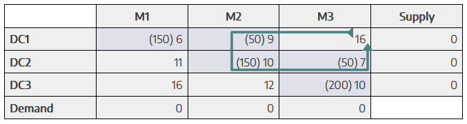
Let us apply the Stepping Stone Method to our example. The following tableau illustrates one such loop identified in the initial solution.
Steps in the Stepping Stone Method:
- Identify All Unoccupied Cells:
These are the potential candidates for improvement. Each unoccupied cell represents a possible new shipping route. - Construct a Closed Loop for Each Unoccupied Cell:
Starting from the unoccupied cell, trace a path through alternating horizontal and vertical moves, connecting only occupied cells, and return to the starting point. The loop must alternate between adding and subtracting units. - Calculate the Net Cost Change for the Loop:
Assign alternating plus (+) and minus (−) signs to the cells in the loop, starting with a plus at the unoccupied cell. Then compute the net change in cost by summing the products of unit costs and their respective signs. - Evaluate All Loops:
-
- If all net cost changes are zero or positive, the current solution is optimal.
- If any net cost change is negative, the solution can be improved. Select the loop with the most negative net cost, adjust the allocations accordingly, and repeat the process.
This method provides a clear and intuitive way to test for optimality and iteratively improve the solution. In the next section, we will demonstrate this process step-by-step using our transportation example.
In the previous tableau, we evaluated the opportunity cost of assigning a shipment to the unoccupied cell (D3/M2). The net cost change associated with this cell was −1, indicating a potential opportunity to reduce the total transportation cost by reallocating shipments through a closed loop.
Interpreting the Negative Opportunity Cost
A negative value (−1) suggests that the current solution could be improved by assigning units to the unoccupied cell (D3/M2). To explore this possibility, we construct a closed loop involving this cell and other occupied cells, following the Stepping Stone procedure.
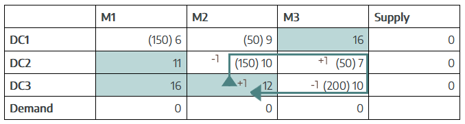
Loop Construction:
The loop formed is as follows:
(D3/M2) → (D2/M2) → (D2 /M3) → (D3/M3)
This loop includes the following cells:
- (D3/M2) (unoccupied, starting point)
- (D2 /M2) (occupied)
- (D2/M3) (occupied)
- (D3/M3) (occupied)
Allocation Adjustments:
We apply alternating +1 and −1 adjustments along the loop:
- +150 units to (D3/M2) (introducing a new shipment)
- −150 units from (D2/M2) (removing the same quantity)
- +150 units to (D2/M3) (reallocating supply)
- −150 units from (D3/M3) (reducing the original allocation)
This reallocation maintains the supply and demand balance while potentially reducing the total cost.
Updated Allocations:
- (D3/M2): 0 → 150
- (D2/M2): 150 → 0
- (D2/M3): 50 → 200
- (D3/M3): 200 → 50
| M1 | M2 | M3 | Supply | |
|---|---|---|---|---|
| DC1 | (150) 6 | (50) 9 | 16 | 0 |
| DC2 | 11 | ( |
( |
0 |
| DC3 | 16 | (150) 12 | ( |
0 |
| Demand | 0 | 0 | 0 |
New Total Transportation Cost:
[latex]\begin{align*} \text{Total Cost} &= (150 \times 6) + (50 \times 9) + (0 \times 10) + (200 \times 7) + (150 \times 12) + (50 \times 10) \\ \text{Total Cost} &= (900) + (450) + (0) +(1400) + (1800) + (500)\\ \text{Total Cost} &= \$5,050 \end{align*}[/latex]
This revised solution results in a reduced transportation cost of $5,050, compared to the original $5,200—confirming that the previous solution was not optimal.
Video: Transportation Method Stepping Stone
Video: "Transportation Method stepping stone" by Professor Dansereau [6:13] is licensed under the Standard YouTube License.Transcript and closed captions available on YouTube.
Finding the Optimal Solution Using the Modified Distribution (MODI) Method
The Modified Distribution Method (MODI) is a powerful optimization technique used to evaluate and improve a basic feasible solution in a transportation model. It relies on the use of dual variables—denoted as Ui for rows and Vj for columns—to calculate the opportunity cost of unoccupied cells and determine whether the current solution is optimal.Let us apply the MODI method to the previously discussed transportation model.
Step 1: Assign Dual Variables Ui and Vj
For each occupied cell (i.e., a cell with a positive allocation), the cost Cij must satisfy the condition:
[latex]Cij = Ui + Vj[/latex]
We begin by arbitrarily setting one of the dual variables to zero. Let U1=0. Using the occupied cells, we solve for the remaining Ui and Vj values.
| V1 | V2 | V3 | |||
|---|---|---|---|---|---|
| D1 | D2 | D3 | |||
| U1 | S1 | (150) 6 | (50) 9 | 16 | 0 |
| U2 | S2 | 11 | (150) 10 | (50) 7 | 0 |
| U3 | S3 | 16 | 12 | (200) 10 | 0 |
| 0 | 0 | 0 |
From the allocations:
[latex]U1=0[/latex]
[latex]\begin{align*} (S1/D1) &= V1 + U1\\ 6 &= V1 + 0\\ V1 &= 6 \end{align*}[/latex]
[latex]\begin{align*} (S1/D2) &= V2 + U1\\ 9 &= V1 + 0\\ V1 &= 9 \end{align*}[/latex]
[latex]\begin{align*} (S2/D2) &= V2 + U2\\ 10 &= 9 + U2\\ U2 &= 10 - 9\\ U2 &= 1 \end{align*}[/latex]
[latex]\begin{align*} (S2/D3) &= V3 + U2\\ 7 &= V3 + 1\\ V3 &= 7 - 1\\ V3 &= 6 \end{align*}[/latex]
[latex]\begin{align*} (S3/D3) &= V3 + U3\\ 10 &= 6 + U3\\ U3 &= 10 - 6\\ U3 &= 4 \end{align*}[/latex]
Final Values:
- U1 = 0
- U2 = 1
- U3 = 4
- V1 = 6
- V2 = 9
- V3 = 6
Step 2: Calculate Opportunity Costs for Unoccupied Cells
For each unoccupied cell, compute the opportunity cost:
[latex]dij = Cij − (Ui + Vj)[/latex]
[latex]\begin{align*} d13 &= 16 - (6 + 0)\\ d13 &= 16 - 6\\ d13 &= 10 \\ \end{align*}[/latex]
[latex]\begin{align*} d21 &= 11 - (1 + 6)\\ d21 &= 11 - 7\\ d21 &= 4 \\ \end{align*}[/latex]
[latex]\begin{align*} d31 &= 16 - (4 + 6)\\ d31 &= 16 - 10\\ d31 &= 6 \\ \end{align*}[/latex]
[latex]\begin{align*} d32 &= 12 - (4 + 9)\\ d32 &= 12 - 13\\ d32 &= -1 \\ \end{align*}[/latex]
Step 3: Check for Optimality
If all dij ≥ 0, the current solution is optimal.
However, since d32 = −1, the solution is not optimal, and there is an opportunity to reduce the total cost by reallocating shipments.
Step 4: Improve the Solution via Pivoting
We construct a closed loop starting at the most negative cell, (S3/D2), and apply alternating + and − adjustments along the loop:
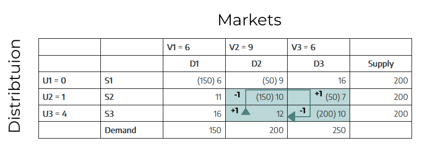
Loop:
(S3/D2) (+) → (S2/D2) (−) → (S2/D3) (+) → (S3/D3) (−)
Revised Allocations:
- (S3 /D2): 0 → 150
- (S2/D2): 150 → 0
- (S2/D3): 50 → 200
- (S3/ D3): 200 → 50
Updated Total Transportation Cost:
[latex]\begin{align*} \text{Total Cost} &= (150 \times 6) + (50 \times 9) + (0 \times 10) + (200 \times 7) + (150 \times 12) + (50 \times 10)\\ \text{Total Cost} &= 900 + 450 + 0 + 1400 + 1800 + 500\\ \text{Total Cost} &= 5,050 \\ \end{align*}[/latex]
This confirms that the MODI method leads to the same improved solution previously obtained using the Stepping Stone Method, validating its effectiveness and accuracy
Video: Transportation Problem Optimal Solution with MODI Method
Video: "Transportation Problem Optimal Solution with MODI Method" by Professor Dansereau [3:58] is licensed under the Standard YouTube License.Transcript and closed captions available on YouTube.
Finding the Optimal Solution Using Linear Programming
The transportation problem can also be formulated and solved as a Linear Programming Problem (LPP). This approach provides a rigorous mathematical framework for minimizing transportation costs while satisfying all supply and demand constraints.
| M1 | M2 | M3 | Supply | |
|---|---|---|---|---|
| DC1 | (X11) 6 | (X12) 9 | (X13) 16 | 200 |
| DC2 | (X21) 11 | (X22) 10 | (X23) 7 | 200 |
| DC3 | (X31) 16 | (X32) 12 | (X33) 10 | 200 |
| Demand | 150 | 200 | 250 |
Decision Variables
Let Xij represent the quantity of goods transported from supply point i (e.g., a distribution center) to demand point j (e.g., a market). Each Xij must be non-negative:
Xij ≥ 0 for all i,j
Objective Function
The goal is to minimize the total transportation cost, which is the sum of the products of unit costs and the corresponding decision variables:
[latex]\text{Minimize Z} = 6X_{11} + 9X_{12} + 16X_{13} + 11X_{21} + 10X_{22} + 7X_{23} + 16X_{31} + 12X_{32} + 10X_{33}[/latex]
Constraints
The model must satisfy both supply constraints (each source cannot ship more than its available supply) and demand constraints (each destination must receive its required quantity):
Supply Constraints:
[latex]X_{11} + X_{12} + X_{13} \leq 200 \text{ Supply from S1}[/latex]
[latex]X_{21} + X_{22} + X_{23} \leq 200 \text{ Supply from S2}[/latex]
[latex]X_{31} + X_{32} + X_{33} \leq 200 \text{ Supply from S3}[/latex]
Demand Constraints:
[latex]X_{11} + X_{21} + X_{31} \leq 150 \text{ Demand from D1}[/latex]
[latex]X_{12} + X_{22} + X_{32} \leq 200 \text{ Demand from D2}[/latex]
[latex]X_{13} + X_{23} + X_{33} \leq 200 \text{ Demand from D3}[/latex]
This formulation captures the essence of the transportation problem as a linear program. The solution to this LPP will yield the optimal allocation of shipments that minimizes total cost while respecting all constraints.
A detailed explanation of how to solve linear programming problems using methods such as the Simplex Method or software-based solvers is provided in the next chapter, Chapter 12: Linear Programming.
