7 Chapter 7

In this chapter we will continue to look at some of the main functions of Microsoft Excel. If you have not yet read Chapter 5 and 6, it is vital that you go back and read it before you continue in this chapter.

• Insert, Move and resize images
  1. Find the Illustrations grouping in the Insert tab and choose Pictures
  2. Click This Device
  3. Search for a picture
  4. The picture is placed into excel. Clicking and holding on the picture will allow you to move it to wherever you want / need in the document. You may wish to insert something like a company logo and place it in the document.
  5. When you click on the image you will see 8 circles surrounding the image in all 4 corners and all 4 sides
  6. Click and hold one of these circles, and drag it to resize the image
• Clear cells and cell formatting
  1. With an Excel Workbook open, enter in the days of the week in cells A1 through F1 (Monday to Saturday)
  2. In cells A2 through F2 put in how many hours you worked each day
  3. Select cells A1 through F1 an d apply Accent 4 as the format under Cell Styles
  4. Select Column F
  5. Find the Editing Grouping in the Home tab
  6. Find the clear button:
  7. Chose the dropdown – you have several options now
     Clear All – this will clear everything out of the cell – formats, contents, comments, notes, hyperlinks. Everything.
     Clear Formats – this will clear only the formatting of the cells
     Clear Conents – this will clear only the contents of the cells
     Clear Comments and Notes – this will clear comments and notes
     Clear Hyperlinks – this will clear hyperlinks
     Remove Hyperlinks – this will remove hyperlinks
  8. Try each of them by clicking them and then clicking the undo button in the quick access toolbar beside the title bar:
• Apply numeric formats and adjust the number of decimal places
  1. In cell K1 type 16.50 as your rate of pay and apply a currency style to it
  2. Find the Number grouping in the Home tab
  3. Look for the Increase and Decrease decimal icons:
     Clicking Increase will increase the number of Decimal Places
     Clicking Decrease will decrease the number of Decimal Places
  4. With cell K1 selected click the decrease button twice
  5. Notice it changes to $17 – this is because anything equal to or over .50 will round up (in this case up to $17), and anything equal to or under .49 will round down (in this case down to $16)
  6. Click the increase button twice to bring the decimal back to 2 decimal places
• Change cell Alignment and indentation
  1. Click in cell K1 with the rate of pay in it
  2. Find the Cells grouping in the Home tab
  3. Click the Format button:
  4. Choose Row Height
  5. Type in 20 – the row height will increase.
  6. Notice that, by default, the rate of pay is left aligned and bottom aligned (it appears in the bottom left corner of the cell)
  7. Find the Alignment grouping of the Home tab
  8. First look for the vertical align buttons:
     The Top Align button will align your data to the top of the cell
     The Center Align button will align your data to the center of the cell vertically
     The Bottom Align button will align your data to the bottom of the cell
     Click Center
  9. Now look for the horizonal align buttons:
     The Left Align button will align your data to the left of the cell
     The Center Align button will align your data to the center of the cell horizontally
     The Right Align button will align your data to the right of the cell
     Click Center
  10. Your rate of pay should now be in the exact center of the cell! Play with the different alignments to see how it changes in the cell.
• Inset and edit comments and notes
  1. First lets discuss the difference:
     Comments are threaded discussions so if you are working with someone on a document you can reply to each other’s comments without having to be there at the same time. You can tell if someone has left a comment as there is a purple comment icon in the top right corner of the cell:
     Notes are more private and are meant to be used on workbooks that you are working on by yourself. They are just notes left in a cell to remind you of something about that cell. You can tell if someone has left a note as there is a red triangle icon in the top right corner of the cell:
  2. Click on the Review tab and notice that there is both a Comments Grouping and a Notes grouping
  3. In the same workbook you’ve been working with, click on cell K1 and leave yourself a note to ask for a raise. Click on the New Note button and write Raise in the note:
     
     Notice that the note includes your first name and last initials, and you can type anything below that. In this case I’ve left a note for me to ask for a raise.
  4. Click on one of the cells you’ve put hours into.
  5. Click New Comment and a popup for the comment will come up:
     
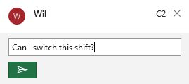
  6. Click the green button to put the comment into the spreadsheet – now the next person who looks at it will notice the comment and hopefully reply to it so you can switch your shift!
• Using Format Painter
  1. In the Home tab find the Clipboard grouping
  2. With cell K1 selected click the Format Painter icon:
  3. Click cell K2 – notice that the format from cell K1 was applied!
  4. In cell K2 type your desired wage (perhaps $17.25)
  5. In cell J1 type ‘Current Wage:’
  6. In cell J2 write ‘Desired Wage:’