Implementing and Analyzing N-Grams in Python
PYTHON IMPLEMENTATION OF N-GRAMS
To implement n-gram analysis, a machine learning model based on NLP is used. (Please refer to the section on n-grams in the previous course for a full explanation of n-grams.) The n-grams are first generated with NLP operations, such as the ngrams() function in the Python NLTK (Natural Language Toolkit) library. For instance, if words is a Python list data structure of words, the operation (note: this example will be presented in further detail below):
nltk.ngrams(words, 2)
returns a zip object of bigrams. To obtain the bigram elements, a Pandas series can be generated from the zip object.
>>> bigram = pd.Series(nltk.ngrams(words, 2))
The bigram series can then be explored.
>>> type(bigram)
<class 'pandas.core.series.Series'>
>>> bigram
0 (much, culture)
1 (culture, pass)
2 (pass, digital)
3 (digital, even)
4 (even, arent)
...
1276 (take, cue)
1277 (cue, technological)
1278 (technological, principle)
1279 (principle, digital)
1280 (digital, artifact)
Length: 1281, dtype: object
The individual elements in the bigram can be accessed either individually, or by slices, like any array.
>>> bigram[0]
('much', 'culture')
>>> bigram[0:10]
0 (much, culture)
1 (culture, pass)
2 (pass, digital)
3 (digital, even)
4 (even, arent)
5 (arent, looking)
6 (looking, screen)
7 (screen, there)
8 (there, good)
9 (good, chance)
dtype: object
For n-grams to be useful, the frequency of each individual word sequence must be known. The Python NLTK supplies the value_counts() function, which is invoked on an n-gram zip object and returns a Pandas series object.
bigram_count = bigram.value_counts()
This object can also be explored.
>>> type(bigram_count)
<class 'pandas.core.series.Series'>
>>> bigram_count[0]
14
>>> bigram_count[1]
13
>>> len(bigram_count)
1207
>>> bigram_count[0:10]
(binary, code) 14
(digital, technology) 13
(0, 1) 11
(page, number) 6
(digital, culture) 5
(code, 0) 4
(event, digital) 3
(sequence, 0) 3
(discrete, code) 2
(technological, determinism) 2
dtype: int64
The bigram frequencies can be accessed directly from the Pandas series. For instance:
>>> bigram_count[0]
14
>>> bigram_count[100]
1
The frequencies can also be put into a Numpy array and explored as follows:
>>> bigram_freqs = np.array(bigram_count)
>>> type(bigram_freqs)
<class 'numpy.ndarray'>
>>> bigram_freqs
array([14, 13, 11, ..., 1, 1, 1], dtype=int64)
The length 2 word sequences can be put into a list with the keys() function, which returns the keys of the Pandas series.
## For clarity, extract the keys from the bigram_count series.
>>> keysBigram = bigram_count.keys()
The resulting data structure of keys can be explored.
>>> type(keysBigram)
<class 'pandas.core.indexes.base.Index'>
>>> keysBigram
Index([ ('binary', 'code'), ('digital', 'technology'),
('0', '1'), ('page', 'number'),
('digital', 'culture'), ('code', '0'),
('sequence', '0'), ('event', 'digital'),
('reading', 'possibility'), ('digital', 'artifact'),
...
('highlevel', 'code'), ('also', 'production'),
('shift', 'direct'), ('digital', 'ontology'),
('mass', 'available'), ('point', 'fixed'),
('art', 'monetary'), ('kindle', 'barnes'),
('number', 'digitized'), ('medium', 'buffeted')],
dtype='object', length=1207)
>>> keysBigram[0]
('binary', 'code')
>>> keysBigram[1]
('digital', 'technology')
>>> keysBigram[1][0], keysBigram[1][1]
('digital', 'technology')
>>> keysBigram[1][0]
'digital'
>>> keysBigram[1][1]
'technology'
Suppose that autocompletion is to be performed on the word “digital”. That is, if w1 is “digital”, the word with the highest probability of occurring after “digital” is to be determined.
>>> w1 = 'digital'
Once the bigram keys have been obtained, the indices of the bigram in which the first word in the tuple is w1 must be obtained. There are multiple correct approaches to this problem. A straightforward approach is to initialize an index list and to iterate through the keys data structure, updating the index list when the first element of the tuple in the current iteration is identical to w1 by appending the iteration index to the index list. This approach can be implemented as follows:
>>> bigram_indx = []
>>> for i in range(0, len(keysBigram)):
if (keysBigram[i][0] == w1):
bigram_indx.append(i)
Another method, which in some cases may be more efficient, is to use a list comprehension. This approach is demonstrated below.
>>> ##Get indices of keys whose first component in the tuple is w1.
>>> indxBigram = [i for i, x in enumerate(keysBigram) if x[0] == w1]
>>> indxBigram
[1, 4, 9, 12, 14, 16, 17, 25, 30, 51, 86, 89, 101, 113, 122, 126, 157, 168, 197, 203, 208, 240, 266, 309, 327, 332, 359, 370, 381, 393, 432, 503, 504, 521, 522, 537, 562, 588, 598, 622, 704, 815, 850, 855, 932, 1032, 1122, 1135, 1174, 1200]
>>> keysBigram[1]
('digital', 'technology')
>>> keysBigram[622]
('digital', 'term')
The same procedure is performed for the unigrams.
## Generate the unigrams.
unigram_count = (pd.Series(nltk.ngrams(words, 1))).value_counts()
## For clarity, extract the keys from the unigram_count series.
keysUnigram = unigram_count.keys()
## Get the indices of keys whose component in the tuple is w1.
indxUnigram = [i for i, x in enumerate(keysUnigram) if x[0] == w1]
>>> indxUnigram
[0]
>>> keysUnigram[0]
('digital',)
>>> unigram_count[0:1]
(digital,) 73
Now, the probabilities can be obtained by converting the frequencies obtained from the bigrams counts and unigram counts to Numpy arrays. The indices just obtained are used to extract the counts of the bigrams and (single) unigram representing the word w1.
>>> p = np.array(bigram_count[indxBigram]) / np.array(unigram_count[indxUnigram])
>>> p
array([0.17808219, 0.06849315, 0.02739726, 0.02739726, 0.02739726,
0.02739726, 0.02739726, 0.02739726, 0.02739726, 0.01369863,
0.01369863, 0.01369863, 0.01369863, 0.01369863, 0.01369863,
0.01369863, 0.01369863, 0.01369863, 0.01369863, 0.01369863,
0.01369863, 0.01369863, 0.01369863, 0.01369863, 0.01369863,
0.01369863, 0.01369863, 0.01369863, 0.01369863, 0.01369863,
0.01369863, 0.01369863, 0.01369863, 0.01369863, 0.01369863,
0.01369863, 0.01369863, 0.01369863, 0.01369863, 0.01369863,
0.01369863, 0.01369863, 0.01369863, 0.01369863, 0.01369863,
0.01369863, 0.01369863, 0.01369863, 0.01369863, 0.01369863])
The sum of the individual probabilities is one (accounting for roundoff error), as expected.
>>> sum(p)
1.000000000000002
The bigrams with the two highest probabilities are:
>>> bigram_count[indxBigram[0:2]]
(digital, technology) 13
(digital, culture) 5
The two most likely words that follow “digital” are “technology” with bigram frequency 13, and “culture” with bigram frequency 5. Therefore, the probability for “technology” following “digital” is 13 / 73 ≈ 0.1781 (recall that the unigram frequency for “digital” is 73, as shown above), and the probability of “culture” following “digital” is 5 / 73 ≈ 0.0685 (to 4 decimal places).
BASIC N-GRAM VISUALIZATION
The following example is based on the web article:
Ednalyn C. De Dios
May 22, 2020
One of the most useful features of n-grams is to analyze how their usage changes in a corpus over time. This is the main function of Google’s Ngram Viewer, discussed previously. In this example, a corpus of news headlines from the website of ABC (Australian Broadcast Corporation) news is investigated through n-grams. The data were obtained HERE. Daily headline text is reported for the period from February 2003 through June 2017, but, for illustrative purposes, the data were combined on a monthly basis. That is, all the headline text for each day in a particular month was aggregated into one large text string, which is subsequently processed with the Python NLTK (Natural Language Toolkit) library. The top 50 unigrams, bigrams, and trigrams were then calculated for each month in each year.
First, the required libraries must be imported.
import numpy as np
import pandas as pd
# Natural language processing: n-gram ranking....
import re
import unicodedata
import nltk
from nltk.corpus import stopwords
# For plotting....
import matplotlib.pyplot as plt
The input file of the headline text, aggregated by year and month, is accessed as a CSV file, and converted to a data frame.
## File I/O....
inputPath = (File Path) ## Specify the correct file path.
## Year/Month aggregation.
inputFileName = 'abcnews-date-text-bydate-yrmo.csv'
inputFile = inputPath + inputFileName ## Full file name, with the path.
## Read the data from the CSV file into a data frame.
df_yrmo = pd.read_csv(inputFile)
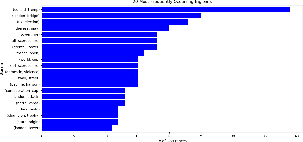
Now n-gram analysis can be applied to the text in the data frame. For example, to analyze the twenty most frequently occurring bigrams for June 2017 (the last available month), the following code is executed.
First, a list of stop words is supplied by the user. These stop words are used in addition to the standard stop words provided by NLTK. Then, the headline text is extracted for the last row in the data frame, corresponding to June 2017. The text is cleaned, as will be described below. The number of most frequently occurring n-grams is selected by the user, twenty (20) in this example. The bigrams are then calculated with the nltk.ngrams() function, invoking the value_counts() function to get the frequencies of the bigrams.
## N-gram analysis....
Nngrams = 20 ## Top 20 bigrams…
# Add appropriate words that will be ignored in the analysis.
ADDITIONAL_STOPWORDS = []
>>> txt = df_yrmo['headline_text'].iloc[-1]
## Obtain a clean set of words from input text....
>>> words = basic_clean(txt)
>>> bigram_counts = (pd.Series(nltk.ngrams(words, 2)).value_counts())[:Nngrams]
The bigram frequencies can now be examined, and plotted.
>>> bigram_counts
(donald, trump) 39
(london, bridge) 25
(uk, election) 23
(theresa, may) 20
(tower, fire) 18
(afl, scorecentre) 18
(grenfell, tower) 18
(french, open) 16
(world, cup) 15
(nrl, scorecentre) 15
(domestic, violence) 15
(wall, street) 15
(pauline, hanson) 15
(confederation, cup) 13
(london, attack) 13
(north, korea) 13
(champion, trophy) 12
(state, origin) 12
(dark, mofo) 12
(london, tower) 11
## Matplotlib plot of the 20 top bigrams....
## Plot size and other characteristics can be modified.
bigram_counts[0:Nngrams].sort_values().plot.barh(color='blue', width=.9, figsize=(12, 8))
plt.title(str(Nngrams) + ' Most Frequently Occurring Bigrams')
plt.ylabel('Bigram')
plt.xlabel('# of Occurences')
## Display the plot....
plt.show(block = False)
The result is shown below. Similar analysis can be performed for unigrams, trigrams, and for different dates, a range of dates, or for all the headlines in the corpus.
The above operation was applied on a cleaned list of words from the corpus. There are many ways to perform this step. The approach taken in this example follows the procedure in “From DataFrame to N-Grams” by E. De Dios, referenced above.
The cleaning process is illustrated below on a text sample named text. First, the NLTK WordNet Lemmatizer is instantiated. NLTK provides a set of frequently used stop words. However, the user can add additional words to a list, ADDITIONAL_STOPWORDS in this case. All the words that are not explicitly designated as stop words as found in the list ADDITIONAL_STOPWORDS are encoded and parsed using standard regular expression parsing. This is followed by obtaining the normal form for the Unicode string text. Specifically, the normal form KD, or NFKD, applies compatibility decomposition. All compatibility characters are replaced with their equivalents. The final encoded text is then normalized to lower case.
The example on text containing Unicode characters is shown below.
>>> wnl = nltk.stem.WordNetLemmatizer()
>>> stopwords = []
>>> text = 'This is an example of WORD LEMMATIZATION...'
>>> text = text + '\u0100 \u0107 \u0133 \u014B \u00FC ....'
>>> text
'This is an example of WORD LEMMATIZATION...Ā ć ij ŋ ü ....'
>>> text = (unicodedata.normalize('NFKD', text)
.encode('ascii', 'ignore')
.decode('utf-8', 'ignore')
.lower())
>>> text
'this is an example of word lemmatization...a c ij u ....'
>>> words = re.sub(r'[^\w\s]', '', text).split()
>>> words
['this', 'is', 'an', 'example', 'of', 'word', 'lemmatizationa', 'c', 'ij', 'u']
>>> cleaned_words = [wnl.lemmatize(word) for word in words if word not in stopwords]
>>> cleaned_words
['this', 'is', 'an', 'example', 'of', 'word', 'lemmatizationa', 'c', 'ij', 'u']
>>>
The following example will display a line graph visualization of unigrams, bigrams, and trigrams as they change over the entire time period, February 2003 to June, 2017. The cleaning process that was described above is performed by the function basic_clean(), as explained Here.
#########################################
##
## Clean the text.
##
#########################################
def basic_clean(text):
#################################################################
##
## Cleaning function found in:
## From DataFrame to N-Grams
## Ednalyn C. De Dios
## May 22, 2020
## https://towardsdatascience.com/from-dataframe-to-n-grams-e34e29df3460
##
## All the words that are not explicitly designated as stop words
## as found in the list ADDITIONAL_STOPWORDS are encoded and parsed
## using standard regex (regular expression) parsing. Following these
## steps, lemmatization is performed with the NLTK
## stem.WordNetLemmatizer() function.
## See:
## https://www.nltk.org/_modules/nltk/stem/wordnet.html
## for additional details.
##
#################################################################
## Instantiate the lemmatizer.
wnl = nltk.stem.WordNetLemmatizer()
## Obtain a standard list of stopwords and add any additional
## stop words provided by the user.
stopwords = nltk.corpus.stopwords.words('english') + ADDITIONAL_STOPWORDS
## Obtain the normal form for the Unicode string 'text'.
## NFKD: The normal form KD, or NFKD, applies compatibility decomposition.
## All compatibility characters are replaced with their equivalents.
## See: https://docs.python.org/3/library/unicodedata.html
## The final encoded text is normalized to lower case.
text = (unicodedata.normalize('NFKD', text)
.encode('ascii', 'ignore')
.decode('utf-8', 'ignore')
.lower())
## Substitute the empty character ('') for any Unicode word characters (\w)
## or Unicode whitespace characters (\s).
## Split the words into a list.
words = re.sub(r'[^\w\s]', '', text).split()
return [wnl.lemmatize(word) for word in words if word not in stopwords]
The last example displayed the twenty most frequently occurring n-grams. For further analysis that may be performed later, this number can be increased, to 50 in this case.
## Number of n-grams
Nngrams = 50
## Obtain the dates from the data frame.
publish_date_yrmo = df_yrmo['publish_date_yrmo']
## Number of dates.
Ndates_yrmo = len(publish_date_yrmo)
Any additional stop words can be specified by the user.
## Define any additional stopwords.
ADDITIONAL_STOPWORDS = []
To facilitate processing, the n-gram counts (frequencies) and the keys, or the sequence of words comprising the n-grams, are stored in a list so that they can be easily appended. Because the frequencies will be normalized by the number of words occurring in the headlines for each date, an additional list is initialized for this purpose. For subsequent processing, the lists are converted to Numpy arrays. This is just one approach. There are other, equally valid methods, and the reader is encouraged to experiment with the code. In this example, unigrams, bigrams, and trigrams are of interest.
## Initialize n-gram counts and keys to a list data structure.
UNIGRAM_COUNTS = []
BIGRAM_COUNTS = []
TRIGRAM_COUNTS = []
UNIGRAM_KEYS = []
BIGRAM_KEYS = []
TRIGRAM_KEYS = []
## Word frequencies (counts) for all dates.
NWORDS = []
The n-gram frequencies and keys are then appended to the lists initialized above.
## Calculate the n-grams in a loop.
for i in range(0, Ndates_yrmo):
## Feedback....
print('Working on ', i, '....')
## Get the text for the i-th date.
txt = df_yrmo['headline_text'].iloc[i]
## Perform cleaning.
words = basic_clean(txt)
## Calculate the n-grams.
unigram_counts = (pd.Series(nltk.ngrams(words, 1)).value_counts())[:Nngrams]
bigram_counts = (pd.Series(nltk.ngrams(words, 2)).value_counts())[:Nngrams]
trigram_counts = (pd.Series(nltk.ngrams(words, 3)).value_counts())[:Nngrams]
## Update the list of the word counts with the count for date i.
NWORDS.append(len(words))
## Update the n-gram counts.
UNIGRAM_COUNTS.append(unigram_counts)
UNIGRAM_KEYS.append(unigram_counts.keys())
BIGRAM_COUNTS.append(bigram_counts)
BIGRAM_KEYS.append(bigram_counts.keys())
TRIGRAM_COUNTS.append(trigram_counts)
TRIGRAM_KEYS.append(trigram_counts.keys())
As indicated above, the lists are then converted to Numpy arrays to facilitate further processing.
###############################################
##
## Convert the arrays to Numpy arrays.
##
###############################################
UNIGRAM_COUNTS = np.array(UNIGRAM_COUNTS)
UNIGRAM_KEYS = np.array(UNIGRAM_KEYS)
BIGRAM_COUNTS = np.array(BIGRAM_COUNTS)
BIGRAM_KEYS = np.array(BIGRAM_KEYS)
TRIGRAM_COUNTS = np.array(TRIGRAM_COUNTS)
TRIGRAM_KEYS = np.array(TRIGRAM_KEYS)
NWORDS = np.array(NWORDS)
Once the n-gram counts and their corresponding keys have been calculated, plots of specific n-grams can be displayed that show how their frequencies change over time. In this example, the focus will be on bigrams. First, the number of bigrams is obtained.
## Obtain the number of bigrams.
N = len(BIGRAM_COUNTS)
The Plotly library will be used to produce an interactive line graph plot.
## Import Plotly for visualizing the n-grams.
import plotly.graph_objects as go
In this example, the user needs to analyze four bigrams to assess their relationships and correlations, for instance: (world cup), (climate change), (wall street) and (mental health). These bigrams are specified as tuples, and stored in a list as follows.
W = [('world', 'cup'), ('climate', 'change'), ('wall', 'street'), ('mental', 'health')]
Now, to display the dates in an intuitive manner, a new list is generated, storing the dates in a format that is easily interpreted by Plotly. Note that since the application only concerns years and months, the day is not relevant, and, for simplicity, is set to “01”.
## Format the dates for display.
dt = [str(a)[0:4] + '-' + str(a)[4:6] + '-' + '01' for a in publish_date_yrmo]
The list can then be examined. For instance, the type of data structure and the first ten dates can be displayed as follows:
## Format the dates for display.
dt = [str(a)[0:4] + '-' + str(a)[4:6] + '-' + '01' for a in publish_date_yrmo]
>>> type(dt)
<class 'list'>
>>> dt[0:10]
['2003-02-01', '2003-03-01', '2003-04-01', '2003-05-01', '2003-06-01', '2003-07-01', '2003-08-01', '2003-09-01', '2003-10-01', '2003-11-01']
The plot can now be generated. A new plot, or figure, is initialized as a Plotly Graphics Object (recall that fig is simply a variable name, and that the user may select a different identifier).
## New figure....
fig = go.Figure()
Now, a separate trace (line graph) is added for each n-gram to the data frame. The counts (frequencies) and keys are obtained from the BIGRAM_COUNTS and BIGRAM_KEYS Numpy arrays, respectively, through a counting function count_ngrams(), parameterized by the bigram counts and keys, as well as the specific n-gram selected by the user. This function simply iterates through each of the n-grams in the list of n-grams for each date and stores the frequency of the n-gram selected by the user by date. Hence, the returned value, called COUNT in this example, contains the frequency for n-gram w at each date (in this case, 173 months from February 2003 to June 2017). Note that to iterate through the list of n-grams for each date t, two alternative methods are shown. The first method is implemented with a while loop, iterating through each n-gram for a specific date t until the n-gram w is matched, or if the maximum number of n-grams for date t have been examined, in which case the n-gram w was not found among the n-grams for date t. The second method is implemented with a for loop, and simply iterates through each n-gram for date t and sets the count if the user-selected n-gram w was found. This method may be slightly less efficient than the first one, as all n-grams for date t must be searched. For instance, if n-gram w is the first n-gram, then, although the count for that n-gram is updated, all the remaining n-grams are still searched. Since each n-gram in BIGRAM_KEYS is unique for a specific date t, this method may be inefficient, especially if a large number of n-grams was calculated. The first method is used in the function definition below, but the second method (with the for loop) is also shown, although it is commented out.
############################################################
##
## Return a count of an n-gram based on a specific key.
##
############################################################
def count_ngrams(NGRAM_COUNTS, NGRAM_KEYS, w):
## Total number of sets of n-grams.
## This is also the number of dates.
N = len(NGRAM_COUNTS)
## There are N dates, and therefore there are N frequencies.
COUNT = np.zeros(N)
## Iterate.
for i in range(0, N):
## Frequencies for n-grams in date i.
counts = NGRAM_COUNTS[i]
## Keys for the n-grams in date i.
keys = NGRAM_KEYS[i]
## Number of n-grams in date i.
n = len(counts)
## Find the n-gram w in the keys.
## Initialize the index variable for the keys.
j = 0
## Increment the index until the key is found, or
## until the end of the n-grams is reached.
while ((j < n) and (w != tuple(keys[j]))):
j = j + 1
## If the word sequence w was found, store its frequency.
if (j < n):
COUNT[i] = counts[j]
################################################
## Alternative method -- loop through all
## the keys, searching for the word sequence.
################################################
## for j in range(0, n):
## if (w == tuple(keys[j])):
## COUNT[i] = counts[j]
## Return the list
return(COUNT)
Returning to the Plotly line plot visualization, a separate trace (line) is added for each n-gram selected by the user for analysis. Recall that the list W contains tuples of these n-grams. The list can contain an arbitrarily large (or small, with a minimum of one) n-grams. The code presented in this example determines the number of requested n-grams with len(W) – although this length can also be stored as a variable for clarity. Note that the y-values for each trace display the normalized frequencies – that is, the raw frequencies for each date that were returned by the count_ngrams() function divided by the corresponding number of words for each date. Also note that the word sequence comprising each n-gram is displayed as a single string, for clarity. The reader should run this code and experiment with it to understand how it works. Of course, the readers are also encouraged to modify the plot for their specific applications. In this example, default colours are used.
## Iterate through all the n-grams of interest....
for i in range(0, len(W)):
w = W[i]
COUNT = count_ngrams(BIGRAM_COUNTS, BIGRAM_KEYS, w)
fig.add_trace(go.Scatter(
x = dt,
y = COUNT / NWORDS, ## The normalized frequencies are needed.
mode= 'lines',
name = ' '.join(w),
showlegend = True,
textposition= 'top center'
))
To make the plot more informative, hover text is added so that if the user hovers over a data point on one or more of the separate traces, the date (x values) and normalized frequency (y values) will be displayed, along with the bigram keys, or sequence of words in the bigram. A legend is also added near the top left corner. Finally, to enhance interactivity, a time/date selector control (also known as a range slider) is added, and is displayed below the plot. This time selector is a powerful feature that facilitates examining a specific time window (“zooming”), thereby enhancing the analysis capabilities of the plot.
## Update the hover template and the position of the legend.
fig.update_traces(hovertemplate = 'Date: %{x} <br>Frequency: %{y}')
fig.update_layout(legend = dict(yanchor= 'top', y = 0.99, xanchor = 'left', x = 0.01),
xaxis_title = 'Date',
xaxis = dict(rangeslider = dict(visible = True), type= 'date'),
yaxis_title = 'Normalized Frequency',
legend_title = 'Bigram'
)
Finally, the plot is displayed.
## Display the plot.
fig.show()
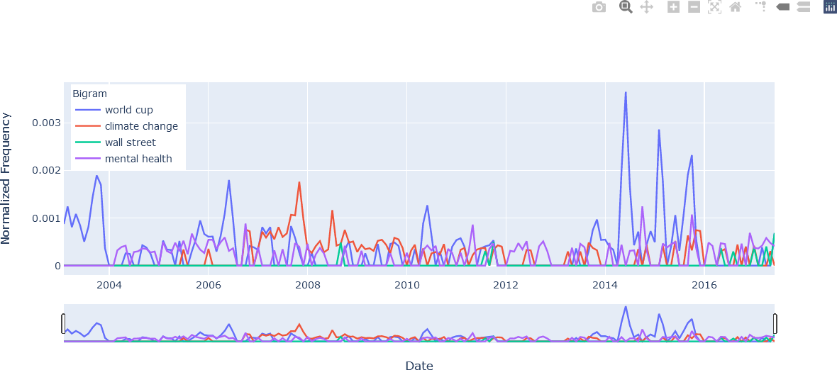
The resulting plots are shown below, illustrating some of their interactive features. By default, the Plotly plot offers controls in the upper right section of the figure. The “Toggle Spike Lines”, “Show closest data on hover”, and “Compare data on hover” features are particularly useful in enhancing analysis capabilities. The reader is encouraged to run the code to obtain similar plots.
The first figure illustrates the appearance of the plot.
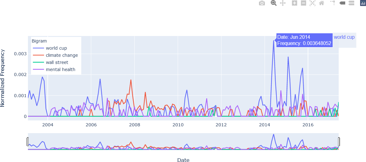
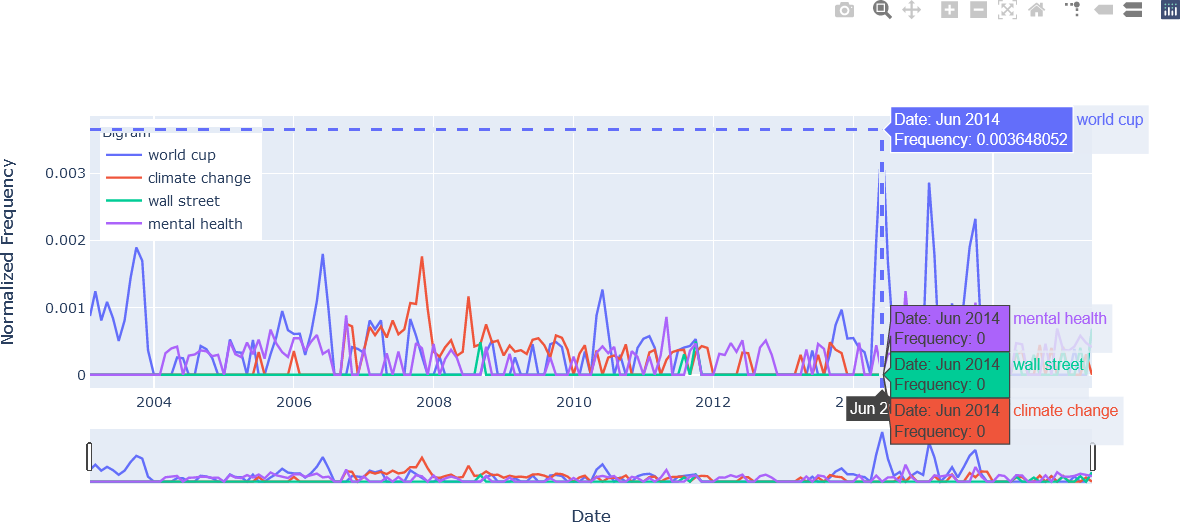
The second figure illustrates the hover text that was added to each trace in the loop shown above. In this example the use of the bigram “word cup” is examined at its highest point in June 2014. Note the appearance of the n-gram text, formatted with name = ' '.join(w).
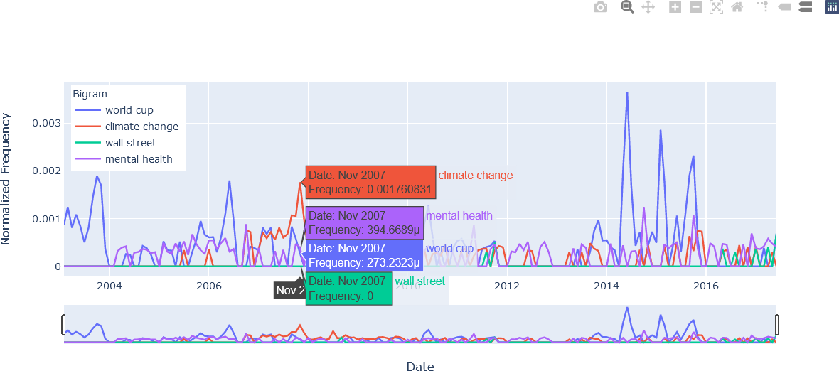
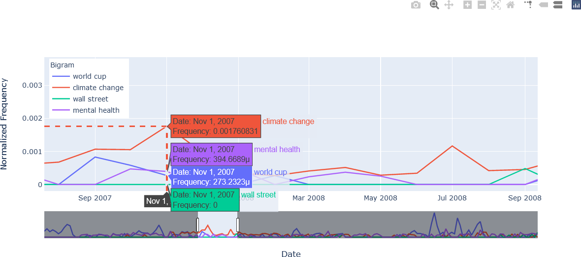
The third figure provides an example of comparing data by hovering over a data point. The m symbol in the hover text for the bigrams “mental health” and “world cup” indicate the value is in terms of one one-millionth, or 10-6. For example, in November 2007, the bigram “mental health” had a normalized frequency of 394.6689 x 10-6 = 0.000395, the bigram “world cup” had a normalized frequency of 273.2323 x 10-6 = 0.000273, and the bigram “wall street” had no occurrences in November 2007 in the corpus of ABC news headlines.
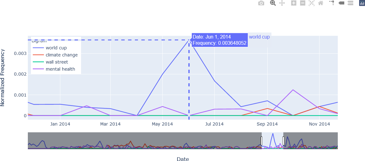
The fourth figure again demonstrates the “Compare data on hover” feature, but in this case spike lines are added to facilitate the view of the coordinate along the axes. In this example, the bigram “world cup” is again examined, and normalized frequencies for the other n-grams specified by the user are also shown. Note that none of the other n-grams were used in this month, as shown in the fifth figure displayed below, which demonstrates using the time selector to limit the time period from December 2013 to November 2014. These plots suggest the dominance of the World Cup event in the headlines from June 2014.
The fifth figure using the time selector to limit the time period from December 2013 to November 2014 is shown below.
The sixth figure again illustrates the time/date selector feature, focusing on the time period from July 2013 to February 2016.
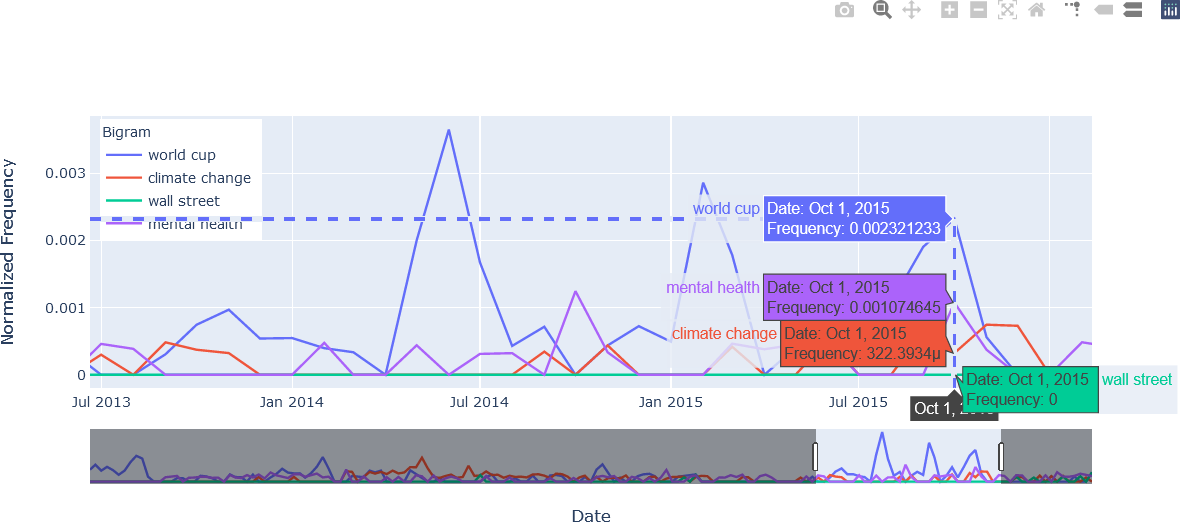
The seventh figure combines the spike lines, compare data on hover, and time selector features.
Finally, as computing the counts and keys (as well as the overall number of words) for the 50 unigrams, bigrams, and trigrams in each of the 173 months is relatively time-consuming, it would be beneficial to save these values for further future analysis. These results can be saved in a Numpy-specific format, or NPZ file, using the Numpy savez() function. In this case, the n-gram counts, keys, and the word count is stored in an output file, abcnews-n-grams.npz, as shown below. The *.npz extension is added by the function, and need not be specified by the user.
#################################################
##
## Save variables.
##
#################################################
nzOutputFileName = 'abcnews-n-grams'
nzOutputFile = inputPath + nzOutputFileName
np.savez(nzOutputFile, UNIGRAM_COUNTS = UNIGRAM_COUNTS,
UNIGRAM_KEYS = UNIGRAM_KEYS,
BIGRAM_COUNTS = BIGRAM_COUNTS,
BIGRAM_KEYS = BIGRAM_KEYS,
TRIGRAM_COUNTS = TRIGRAM_COUNTS,
TRIGRAM_KEYS = TRIGRAM_KEYS,
NWORDS = NWORDS)
