Artificial Neural Networks
INTRODUCTION
Artificial neural networks (ANNs), or simply neural networks, are the most popular supervised machine learning technique, and are particularly useful for classification. ANNs are connectionist models, wherein nodes, or neurons, compute values based on their input, and send their computed values to other nodes for further processing. In a very general sense, ANNs accept input, transform it, and calculate output. However, the goal of ANNs is not simply to compute function values, but to compute values that match some desired output. ANNs are mathematical models in machine learning that are “trained” to produce outputs specified by a human user. For instance, in medicine, numerical metrics measured from a patient, such as blood pressure, blood glucose, pulse rate, temperature, etc., can be input into an ANN, generating as the output whether the patient has a certain condition, such as the flu. More specifically, the output of the ANN may be the probability that a person has the flu, where the probability ranges from 0 to 1. For the ANN to recognize a patient’s condition based on medical measurements, it must be trained. Combinations of measurements from a large number of patients that are known to either have the flu or not have it are labeled by a human user. The ANN is presented both the clinical measurements as input, and the label (flu/no flu) as output. This set of data, consisting of input values and labels, is known as training data. The ANN then attempts to “learn” the function that transforms the medical measurements (input) into output (flu/no flu), based on the label supplied by the human user. To achieve this goal, the ANN is “trained” to “learn” this function. The training process is an iterative process, meaning that the ANN transforms the input into output through a mathematical model, compares the output to the labels (the “correct” values) supplied by the human user, and a adjusts the model to gradually achieve the correct outputs over time. Each iteration is sometimes called a generation. In a more complex example, an ANN may be trained to recognize several disease conditions, and not just one. The training process consists in the ANN adjusting its internal mathematical model so that the difference between its output and the desired output supplied by the user is minimized. As the labels are supplied by a human user, ANNs are a supervised learning approach.
As mentioned, ANNs are a connectionist model. An ANN is a network of interconnected nodes that perform simple computations based on an input and send the computed output to other nodes. However, the neurons that comprise the network are arranged in a specific way. Neural networks consist of layers, or groups of neurons. ANNs consist of three or more layers. An input layer contains nodes for each numerical value of the input vector. For example, if an ANN is to be trained to recognize three disease states based on five clinical measurements, say, temperature, blood pressure, pulse rate, respiration rate, and red blood cell count, then the input layer has five neurons, one for each measurement. The input layer is connected to a hidden layer. Specifically, the neurons in the input layer are connected to the neurons in the hidden layer. Each neuron in a hidden layer is called a hidden neuron, or hidden unit. The number of hidden neurons in the hidden layer is generally higher than the number of neurons in the input layers. The hidden layer is connected to the output layer – that is, the neurons in the hidden layer are connected to neurons in the output layer. The number of output layer neurons depends on the problem being solved. In the current example, if one of three disease states is to be determined, then the output layer will have three neurons. In the previous example, where a binary decision of flu/no flu is to be calculated, the ANN needs one output neuron. ANNs are generally, but by no means always, fully connected. That is, every input neuron is connected to every hidden neuron, and every hidden neuron is connected to every output neuron.
In that case, if an ANN has Ninput input neurons in the input layer, Nhidden hidden neurons in one hidden layer, and Noutput neurons in the output layer, then there are (Ninput)(Nhidden) connections between the input and hidden layers, and (Nhidden)(Noutput) connections between the hidden and output layers.
These concepts are illustrated by the figure below.
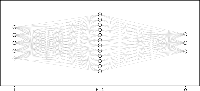
In this case, since five clinical measurements are used (four clinical vital signs and red blood cell count), there are five neurons in the input layer. This particular ANN has one hidden layer with twelve hidden neurons. Because one of three disease states (or two disease states and a no disease state) is to be identified, there are three neurons in the output layer. There are (5)(12) = 60 connections between the input and hidden layers, and (12)(3) = 36 connections between the hidden and output layers, for a total of 60 + 36 = 96 connections in this particular ANN.
Values computed by the input layer are sent to the hidden layer, which uses these values as input. Each neuron in the hidden layers performs computations on the inputs it receives, and sends the resulting calculations to the output layer. Because the input layer neurons send their outputs to the hidden layer neurons, which subsequently send their outputs to the neurons in output layer, this type of ANN is known as a feedforward artificial neural network, or simply as a feedforward network.
Many practical classification tasks can be solved with ANNs with a single hidden layer. However, in recent research into ANNs, complex classification and image recognition problems employed additional hidden layers. These ANNs are called deep artificial neural networks, and the “learning” or optimization of these deep ANNs is referred to as deep learning. An example of a deep ANN is shown below. This ANN has an input layer with seven neurons, three hidden layers with twelve, fifteen, and eight neurons respectively, and four output neurons. Assuming that the network is fully connected there are therefore (7)(12) = 84 connections from layer I to layer HL 1, (12)(15) = 180 connections from layer HL 1 to layer HL 2, (15)(8) = 120 connections from layer HL 2 to layer HL 3, and (8)(4) = 32 connections from layer HL 3 to layer O. There are therefore 84 + 180 + 120 + 32 = 416 connections in this ANN. It must be remembered that these neurons are not physical hardware devices. They simply compute a simple function value based on their input, which is weighted, as explained below. This output function value is then transformed, and sent to the subsequent layer of the network.
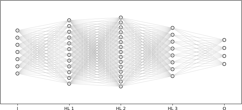
The column of four neurons, denoted as black unfilled circles on the right represent the output layer labeled “O” on the plot. Light grey lines connect all the neurons in the input layer to all the neurons in the first hidden layer. Light grey lines connect all the neurons in the first hidden layer to all the neurons in the second hidden layer. Light grey lines connect all the neurons in the second layer to all the neurons in the third hidden layer. Light grey lines also connect all the neurons in the third hidden layer to all the neurons in the output layer.
ANNs have a long history in computer science. Their mathematical pre-history reaches back into the late nineteenth century. “Computational machines” that implement some aspects of ANNs have been proposed and implemented in the first half of the twentieth century. However, the invention of the perceptron in 1958 by American psychologist Frank Rosenblatt is generally considered as the first modern ANN model. The perceptron is not a device or piece of hardware. It is an algorithm for supervised learning that implements what is known as a binary classifier, which is a function that determines whether a set, or vector, of numbers belongs to a particular class or category. In other words, the perceptron is a multi-valued function that is provided with numerical input and calculates a binary value to indicate whether these numbers belong to a user-specified class. The perceptron algorithm was modeled on the understanding of neural connections in the brain. Most ANNs that are currently in use are still based on the perceptron model. A large class of feedforward neural networks use multiple layers of perceptrons, such as layers for input, output, and hidden layers. These feedforward networks are called multilayer perceptrons (MLPs). In classification problems, the values in the output layer are often probabilities, the highest of which determines the output label that the network calculates. For instance, in the three-disease state ANN example described above, the three output neurons corresponding to the three disease states each contain probability values. The sum of the three probabilities is 1.0, or close to 1.0 due to possible roundoff error. The final output is the label corresponding to the output neuron with the highest probability value.
As stated above, since the early 2000s, there has been a burst of activity and interest in ANNs, particularly because of their success in image and video recognition applications using deep ANNs. ANNs and their applications have an interesting history, and the reader is encouraged to study some and of the tutorials and introductions to ANNs that are available on the Web. The section on the history of neural networks on E. Roberts’ tutorial site is a good place to start.
Artificial neural networks are used in a variety of applications in the digital humanities. Among the many humanities applications represented in the literature, ANNs have been used for investigating historical images (Wevers & Smits, 2020). Advanced ANN architectures have been proposed for text analysis for obtaining semantic information from texts (Ying & Huidi, 2020), for identifying poets based on input text (Salami & Momtazi, 2021), and for facilitating sentiment analysis for decoding memories of the Holocaust (Blanke et al., 2020). Deep neural networks have also been employed for text analysis (Suissa et al., 2021). Research into deep ANN architectures for natural language processing – an important component in many fields of digital humanities scholarship – is also an active area (Li, 2017). Additionally, deep artificial neural networks are used in optical character recognition (OCR). OCR of historical documents is an important topic in the digital humanities, and large-scale projects have been undertaken to improve the usability and accessibility for non-technical scholars. Systems to facilitate this work usually includes graphical interfaces that incorporate OCR into workflows, which include image optimization, page layout analysis, and automatic post-OCR correction (Drobac & Lindén, 2020). A variety of customizable open-source tools for OCR have used advanced ANN architectures, such as one-level long short-term memory (LSTM) networks, a type of network with feedback connections. New tools and some newer versions of established systems are now trained with deep neural networks (Drobac & Lindén, 2020). As a very basic example of an application that can be used with OCR, an illustration of training a simple ANN architecture to recognize small images handwritten digits is presented below.
THE ANN MATHEMATICAL MODEL
ANNs are mathematical models that accept input and generate output. They are “trained” by iteratively optimizing, or minimizing, the error between the “true” labels or classes supplied by the human user and its own output. Network “training” is an iterative process, occurring over several generations. During this training, the mathematical model is being optimized to reduce this error. There are several ways to compute this error. A simple method is sum of squared errors. The difference between the user supplied label (the error) is calculated and squared for each output neuron. The squared errors are then summed together, and this sum indicates how well or poorly the output of the networks corresponds to the true, human-supplied labels. An optimization (minimization) algorithm is then applied to adjust the model parameters, and the process is iterated. The model is re-run on the same input data, resulting in new outputs because of the adjusted model. The error metric is recomputed, and the process continues. Network training is said to converge if the error becomes small enough, usually by reaching a user-specified threshold value. Training ends when the network training converges (the error metric between the output of the network and the user-specified values) falls below a pre-specified threshold for the error, or if a maximum number of generations has been reached. The error threshold and the maximum number of generations are both specified by the user, and are considered to be hyperparameters. However, if training does not result in an acceptable error metric in the given number of generations, then the resulting network will be inaccurate. In this case, the user may decide to modify various network hyperparameters, or adjust the number of hidden neurons or even the number of hidden layers.
From the preceding discussion, it is seen that, in very basic terms, artificial neural networks transform input into output. Because the output of the network is fundamentally calculated from transformed weighted sums of input values and weight parameters, artificial neural network models are large, complex functions. In fact, ANNs are universal function approximators. In other words, given any function f(x) that takes an input vector x, where x can have any number of dimensions, there is a neural network that can be constructed that approximates f(x). For example, in 2D, consider the function f(x, y) = x + y. (Here, x is the vector [x, y]). Because ANNs are universal function approximators, an ANN can be constructed and train to approximate x + y given these two input values. Mathematically proving this property of neural networks is very complex and will not be presented here. However, the universal approximation property of ANNs illustrates the power, versatility, and usefulness of this supervised machine learning approach. ANNs can therefore be used for many applications beyond classification, including regression (fitting a model through a set of observations) and determining complex relationships between predictor values (inputs) and responses (outputs) in large, high dimensional systems.
NETWORK PARAMETERS
The most important parameters of the ANN model are the weights associated with each connection to each neuron. Neurons receive input values, either from user-supplied input if the neuron is in the input layer or from other neurons if the neuron is in hidden layers or the output layer. This value is then multiplied by another number, known as the weight, which is associated with the connection leading into the neuron. If a neuron receives values from n other neurons, then there are n weights. Each input value into a neuron is multiplied by the weight of the connection for that input value. All the input values are multiplied by their associated weights and summed together. Therefore, the neuron computes a weighted sum of the input values it receives and the weights associated with each connection.
For example, consider an ANN with two input neurons in the input layer, four neurons in the hidden layer, and one output neuron in the output layer. Each input neuron has one weight associated with the user-supplied input. In other words, the input value supplied by the user to a neuron is multiplied by the weight associated with that neuron. The same is true for other input neuron in the ANN. The input layer therefore produces two weighted sums.
Before the two input neurons send their output to the hidden layer, the weighted sums undergo a mathematical transformation. That is, some function is applied to the weighted sums. This function is known as an activation function. The most basic activation function is the linear function: y = x. In other words, the weighted sum remains unchanged after transformation. The rectified linear unit activation function, or ReLU, is a more complex linear activation function that is often used in ANN training. However, nonlinear functions are more useful for ANN training. A common nonlinear activation function is the sigmoid function, which transforms inputs into values ranging from 0 to 1. Other nonlinear activations exist as well, such as the softmax function, which is also widely used. The activation used in network training is a hyperparameter specified by the user. The input layer and each of the hidden layers can have different activation functions. ANN implementations in Python (Scikit Learn) offers a selection of activation functions. The mathematical details of these functions are beyond the scope of the current discussion, but the interested reader is referred to This and This for further details.
Now, consider the neurons in the hidden layer. Each hidden neuron receives two inputs – one from each input neuron. That is, each hidden neuron receives the output of each input neuron as its own input. Since there are two connections to each hidden neuron (because there are two input neurons), there are two weights. For each hidden neuron, the two input values are multiplied by the weights corresponding to each of the two connections. Therefore, each of the four hidden neurons receives two inputs, and multiplies these inputs by the corresponding weight of the connection, sums the values to calculate a weighted sum, and transforms the weighted sum through the activation function.
Therefore, the weights are the parameters of the ANN. At the start of training, they are random numbers assigned to the network connections. They are updated by the training process (optimization algorithm). Recall that parameters of machine learning algorithms are updated during training, but hyperparameters are not. The number of hidden layers and the number units in each layer, the activation function(s), the maximum number of training generations, the error threshold, and other values such as the learning rate, are hyperparameters and are not modified during network training.
ANN TRAINING
ANN training is technically an optimization process. An optimization (minimization) algorithm is run to update the weight parameters of the network connections, as discussed above. In fact, one reason that nonlinear activation functions are often preferred for training ANNs is that they facilitate optimization. Specifically, the ANN is a mathematical model consisting of a set of equations (functions) representing neurons. These neurons calculate function values (outputs) based on their inputs and parameters (the weights) of these functions. The goal of training (optimization) is to determine the weights that minimize (optimize) the error between the values in the output layer and the user specified training values. Mathematical optimization is an extremely large and complex field and is crucially important in machine learning. For basic feedforward neural networks, the preferred optimization approach is called backpropagation (or back propagation). In backpropagation, the weights of the connections in the ANN are adjusted starting at the output layer, and “propagating” back to the connections from the input layer neurons to the hidden neurons in the first hidden layer. This optimization process is iterative. It is a process that takes place over several generations of training, ideally reducing the error in each generation until an acceptable error is achieved. Backpropagation uses the mathematical concept of derivatives, specifically gradients, to efficiently adjust the network weights to minimize the error between the ANN output and the user specified training values. The details of backpropagation are very complex mathematically and are beyond the scope of the current discussion. Backpropagation and other optimization techniques used in machine learning are implemented in most programming languages as library functions. Many of these techniques are implemented in the Scikit Learn library for Python.
ANN training is a computationally intensive process, due to the complexity of numerical optimization and the number of connections. This complexity is one of the reasons that deep learning is a relatively new technique, as improvements in hardware enabled its efficient use. For instance, in the deep ANN shown above with three hidden layers, there are 416 connections, and therefore 416 weights must be updated, making the optimization a 416-dimensional problem. Such a problem taxes typical CPUs. With the increased use of programmable, general purpose graphics processing units (GPUs) and multicore processors that provide parallel computing capabilities, deep ANNs can be trained efficiently, and consequently, applications that were formerly excessively time-intensive have become feasible. These applications include image recognition problems with large images that require hundreds of hidden neurons, and possibly many hidden layers.
To summarize, ANN training consists of minimizing the error between the network outputs and the labels in the training data. This optimization – specifically minimization – process consists of iteratively adjusting the weights on the network’s connection until an acceptable error is achieved, or until a maximum budget of training generations has been expended.
VALIDATION AND TESTING
In constructing, training, and analyzing ANNs for a specific task, the available user-specified data is usually split into training data and validation data. Validation is the process of presenting new data to the network to test the effect of the hyperparameters, such as the number of hidden neurons. As validation is associated with tuning the hyperparameters, it is usually performed after the ANN has been trained. When the hyperparameters are tuned, the ANN must be re-trained to obtain a new set of parameters (weights) that minimize the error of the ANN. Many statistical approaches can be used for determining the ratio of training data to validation data, and how to iteratively perform training and validation. These techniques are available in ANN implementations in a variety of programming languages. Once the hyperparameters have been tuned and the ANN trained, resulting in an optimal set of weights, the network is tested. Testing consists of presenting the trained and validated ANN with new data, called testing data, that has not been used in training or validation. Testing is an essential part of ANN analysis. As the testing data is labeled by the user, an analysis can be conducted on how the network performed on “unseen” data, or data on which it has not been trained or validated. In other words, how well the ANN generalizes to correctly classify new data is assessed. If an ANN generalizes well, it produces accurate output for new data. As explained in the introductory section on machine learning, if the network suffers from overfitting, it “memorized” the input data and the corresponding label, and, although it produces highly accurate results for the data on which it has been trained and validated, it performs poorly on new data. Overfitting often occurs when the training data contains noisy, or inaccurate observations, or if the ANN is too complex. For example, it may have too many parameters, such as an excessive number of hidden neurons, and therefore too many weights for the connections. Overfitting is a common problem in supervised machine learning algorithms, and a variety of techniques are available to avoid it.
A SIMPLE NEURAL NETWORK IMPLEMENTATION
A simple Python implementation of an ANN classifier using Scikit Learn is described below. Functions for constructing, training, testing, and analyzing ANNs are described Here. Specifically, the ANN in this example will utilize multilayer perceptron (MLP) functions. An MLP architecture is a reasonable ANN model choice for this example, although other ANN architectures, including deep ones, could be investigated. The reader is encouraged to experiment with these different architectures, and to compare the results with those presented here.
The example uses a canonical data set that is frequently used to demonstrate ANN concepts and to test new ANN architectures and algorithms. The data set comes from of a large database of small images of handwritten characters, known as the MNIST (Modified National Institute of Standards and Technology) database. The images are generally greyscale, meaning that they contain values ranging from 0 to 255 for 8-bit representations, or scaled to the range 0 to 1. Black (or dark) characters are displayed against a white (or light) background. The images have been sized to 31 rows and 36 columns. Therefore, each image contains (31)(36) = 1116 pixels (picture elements). The example presented here focuses on handwritten numerical digits from 0 to 9. Some examples of these handwritten digits are shown below for characters 0, 7, and 8.
Functions for constructing and training the ANN are first imported. (NOTE: The source code for this example is in the file ANN_MNIST_Example.py, which is included in the distribution for this course.)
## Numerical functions....
import numpy as np
## Functions for displaying images....
import matplotlib.image as mpimg
## ANN multi-layer perceptron classifier....
from sklearn.neural_network import MLPClassifier
## Functions for splitting the data into training
## and testing sets....
from sklearn.model_selection import train_test_split
## Functions to facilitate file I/O....
from os import listdir
from os.path import isfile, join
## For flexibility in handling warnings....
import warnings
The number of labels (digits) and the number of images are set.
## Number of labels....
Ndigits = 10
## Number of images for every label....
NsamplesPerDigit = 400
The Python script ANN_MNIST_Example.py includes code to read the images from a specified directory and to preprocess the images so that they can be used in the ANN functions. The reader is encouraged to study this preprocessing code, and to modify it, as necessary.
The original MNIST images were obtained from the GitHub page. The name of each file contains the name of the digit it represents, and therefore the labels for each image are readily accessible. Preprocessing consists of reading the images, scaling the 8-bit pixel values to the range 0 to 1, flattening each image to an array of 1116 pixel values (i.e., the 2D 31 row by 36 column images are rearranged so that their values are in a 1D array with 1116 elements), and placing these pixel values for each image into a 2D Numpy array. In this experiment there are 4000 such images, in which each of the ten digits is represented with 400 images.
After the images have been preprocessed, it is assumed that the data are stored in a 2D Numpy array X with 4000 rows (one row for each image) and 1116 columns (the number of pixels in each image). The labels, obtained directly from the name of the file, are stored in the list y. The dimensions of these variables can be verified.
>>> type(X)
<class 'numpy.ndarray'>
>>> X.shape
(4000, 1116)
>>> type(y)
<class 'list'>
>>> len(y)
4000
The image data and the labels are then split into testing and training sets with the train_test_split() function imported above from the Scikit Learn package. The number of samples for training and testing are stored in variable names for later use.
#########################################################################
##
## Split the data into training and testing sets, and
## train the classifier....
##
#########################################################################
print('Preparing ANN and classifying....')
X_train, X_test, y_train, y_test = train_test_split(X, y,
stratify = y,
random_state = 1)
## Number of training and testing samples....
Ntrain = len(X_train)
Ntest = len(X_test)
The function call split the data into 3000 samples for training and 1000 samples for testing. Other splitting methods are also available. Refer to This for further details.
>>> Ntrain
3000
>>> Ntest
1000
The training and testing data remain 2D Numpy arrays, and the training and testing labels remain lists.
>>> X_train.shape
(3000, 1116)
>>> len(y_train)
3000
>>> X_test.shape
(1000, 1116)
>>> len(y_test)
1000
In this example, the maximum budget of training iterations (generations) is set to 1000. The ANN will have one hidden layer. The number of hidden layers and hidden neurons in each layer, as well as the maximum number of generations, are hyperparameters selected by the user. In this case, because of the size of the images, a large number of hidden neurons, 256, is selected.
## Maximum number of iterations (generations) for ANN training.
MAX_TRAINING_ITERATIONS = 1000
## Number of hidden neurons. This number should be large
## because of the size of the input data.
nHiddenNeurons = 256
The ANN is shown graphically below.
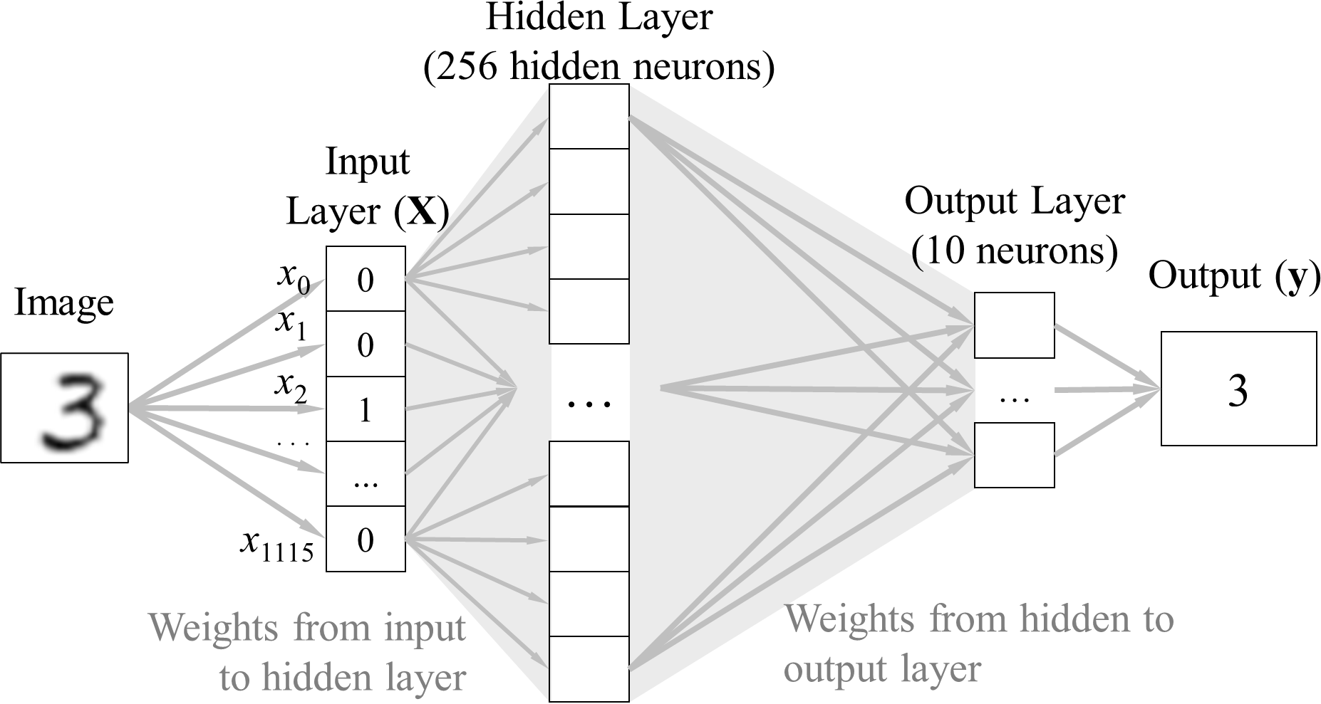
The construction and training of the ANN is accomplished with the Scikit Learn MLPClassifier class. The hyperparameters that are used to construct the network were defined above. The network is trained on the training data with the fit() function. The goal of the training is for the ANN mathematical model to minimize the error between the output values of the network (which are based on the input training data and the connection weights) and the training labels supplied by the user. As discussed above, the training is accomplished through optimization that iteratively updates the connection weights to minimize the error. Note that the hidden_layer_sizes hyperparameter setting is set to one hidden layer with nHiddenNeurons (= 256) hidden neurons through the singleton tuple (nHiddenNeurons, ). Multiple hidden layers with different numbers of hidden neurons can also be specified as a tuple. For example, the hyperparameter setting hidden_layer_sizes = (200, 100, 300) constructs an MLP ANN with three hidden layers, with 200, 100, and 300 hidden neurons in the first, second, and third hidden layer, respectively.
See Here for further details on these functions.
## Initialize the classifier, and train with the training data and labels.
clf = MLPClassifier(random_state = 1, max_iter = MAX_TRAINING_ITERATIONS,
hidden_layer_sizes = (nHiddenNeurons, )).fit(X_train, y_train)
The ANN object is represented by the clf variable name. The ANN can be explored through its member functions. In the IDLE interface, entering clf at the command prompt and pressing the tab key presents a list of methods (functions) and attributes from which the user can select.
>>> type(clf)
<class 'sklearn.neural_network._multilayer_perceptron.MLPClassifier'>
>>> clf.hidden_layer_sizes
(256,)
>>> clf.solver
'adam'
>>> clf.learning_rate_init
0.001
>>> clf.learning_rate
'constant'
From these command line queries, clf is an MLPClassifier object. Attributes of the network can be determined, and methods specific to MLP classifiers can be run on this object. There are 256 hidden neurons in the single hidden layer is, as specified by the user. In this example, many network defaults were used. For example, the training process uses the “adam” numerical optimization algorithm. The learning rate is initially set to 0.001, and remains constant throughout training. Some training algorithms adaptively adjust the learning rate as the training progresses. The interested reader can refer Here for further details on defaults and hyperparameter settings.
Multiple hidden layers for deep learning are also supported. For instance, the following code generates a neural network with three hidden layers, with the numbers of hidden neurons in each layer specified (200, 100, 300, respectively).
>>> clf1 = MLPClassifier(random_state=1, max_iter = MAX_TRAINING_ITERATIONS,
hidden_layer_sizes = (200, 100, 300))
>>> clf1.hidden_layer_sizes
(200, 100, 300)
Recall the Scikit Learn function specified above.
## Initialize the classifier, and train with the training data and labels.
clf = MLPClassifier(random_state = 1, max_iter = MAX_TRAINING_ITERATIONS,
hidden_layer_sizes = (nHiddenNeurons, )).fit(X_train, y_train)
Note that this code not only creates the network with the user specified hyperparameters (or defaults), but also performs training through the fit() function, invoked on the clf ANN object. When the function completes, the network is trained, and testing can begin.
First, the training error is computed by comparing the labels output by the network from the training data with the training labels provided by the user during training. In other words, this step assesses how well the network was trained. The predict() method (function) is run on the clf ANN object with the training data, and the labels calculated by the network are returned into the variable name y_train_predict.
## Calculate the training performance.
y_train_predict = clf.predict(X_train)
To find the ratio of labels correctly calculated by the ANN, the number of correct labels is determined with the Boolean equality operation, divided by the total number of training samples.
y_train_corr = sum(y_train_predict == y_train) / Ntrain
>>> y_train_corr
0.9976666666666667
In this example, the training resulted in almost 100% correct labels, with 2993 out of 3000 images correctly labeled.
>>> sum(y_train_predict == y_train)
2993
The network appears to be trained well. However, the network may have “memorized” the training data, and may not be able to generalize to correctly label unseen inputs, or images on which the network has not been trained. Therefore, assessing the testing performance is crucial. The predict() function is again run on the ANN object, but this time with the testing data, which has not been “seen” by the network during training. The ratio of correct labels is calculated in the same way as with the training data.
## Calculate the testing performance.
y_test_predict = clf.predict(X_test)
y_test_corr = sum(y_test_predict == y_test) / Ntest
>>> sum(y_test_predict == y_test)
864
>>> y_test_corr
0.864
In this case, 864 out of the 1000 training images were correctly labeled, for a ratio of 0.864 correct. This success rate is obviously lower than for training, but that is to be expected, as the ANN is encountering data on which it was not trained. In general, the 0.864 success rate of this network can be considered acceptable for many non-safety-critical applications. For medical, clinical, or safety-critical operations, this success rate would likely be considered too low. However, whether the success rate is “good” is highly dependent on the application and on the user.
To explore the output layer, the user can obtain the probability values of each of the ten output neurons (one output neuron for each label) for any sample. Recall that the labels produced by the network were stored in the variable y_test, which is a list of length Ntest, which is 1000 in this example. The probabilities computed by each output neuron can be observed with the predict_proba() function, which is a method (member function) of the MLP ANN object. This function is run on the clf object, and parameterized by the testing data, X_test.
p_test = clf.predict_proba(X_test)
>>> type(p_test)
<class 'numpy.ndarray'>
>>> p_test.shape
(1000, 10)
It is seen that the function returns a 2D Numpy array with 10 values (corresponding) to the output neurons for each of the 1000 testing samples. For example, the probabilities for the 0th sample can be directly accessed as follows (Note: The reader may obtain different values due to the random number generator on the reader’s system).
>>> p_test[0]
array([7.89275154e-05, 7.05495574e-03, 3.69140888e-03, 1.28354480e-04,
1.34328840e-05, 1.09742322e-02, 4.13695239e-01, 1.87388176e-08,
5.64363399e-01, 3.18346371e-08])
A list of 10 probability values is returned. The sum of these probabilities is approximately 1.0. It is also observed that the 8th probability value is the highest.
>>> np.sum(p_test[0])
0.9999999999999999
>>> pmax = np.max(p_test[0])
>>> pmax
0.5643633986048644
>>> np.argwhere(p_test[0] == pmax)
array([[8]], dtype=int32)
This result corresponds to 0th label, which is 8. In other words, as evidenced by the probabilities computed by the network, based on the input values of the 0th image, the ANN classified that image as the digit “8”.
>>> y_test[0]
8
CONCLUSION
Basic artificial neural network concepts were presented and illustrated with a simple example of handwritten digit classification (labeling). Network performance was determined by the success rate, or the ratio of correctly labeled images. In the next section, additional and more detailed analyses will be presented to assess network performance.
EXERCISE
Try to improve the testing performance of the network (i.e., achieve a success rate greater than 0.864) by adjusting the hyperparameters. Is the number of hidden neurons too high or too low? Are additional hidden layers needed? Would training benefit from a different numerical optimization method, or with a different learning rate or learning adaptation (rather than keeping the learning rate constant)? Proceed with caution, however. Adding an excessive number of hidden neurons or additional hidden layers greatly increases the training time, and may not significantly improve performance.
