9.4 Interpreting Expected Return and Standard Deviation
Learning Objectives
- Assess the expected return and risk of different investment opportunities using the concept of expected return, standard deviation, and risk aversion to make informed investment decisions.
- Distinguish between diversifiable (firm-specific) risk and non-diversifiable (market) risk, explaining how diversification can reduce overall portfolio risk.
- Compare different investment options by analyzing the trade-offs between expected return and associated risks, considering factors such as individual risk aversion and market conditions.
The expected return gives us an idea of how much we will make on the investment. Remember that it is not how much we will make but how much we would make on average if we could repeat the holding period an infinite number of times. Think of a situation where you are asked to pick a number between [latex]1[/latex] and [latex]10[/latex]. If you select the correct number you get [latex]\$100[/latex] and if not you get nothing. Any time that you try this, you will either receive [latex]\$100[/latex] (if you are lucky) or [latex]\$0[/latex]. However, if you could repeat the exercise [latex]100,000[/latex] times, you would find that you would make almost exactly [latex]\$10[/latex] per time. It is critical to know expected values when selecting investments. For instance, if someone offered you the opportunity to do this exercise for [latex]\$9[/latex] per pick, and you could pick as often as you wanted, it would be an excellent opportunity. Alternatively, if you were offered the same thing for [latex]\$11[/latex], you would (hopefully) walk away. However, it is just as important to understand that the expected return is only an average return and not the return you will receive in any particular instance. This example also illustrates why it is so important to focus on the process and not the result. If you had the opportunity to play this game once for a cost of [latex]\$2[/latex] and you lost, it still was a smart decision to play and you should do it again if you got the chance. If you had the opportunity to play this game once for a cost of [latex]\$20[/latex] and you won, it was still a bad decision to play and you should pass if offered the opportunity to try again.
Example 9.4.1
Example 9.4.2
Let's put this in financial terms. Consider two stocks.
- Stock A has an expected return of [latex]10\%[/latex] and a standard deviation of [latex]25\%[/latex]. Stock B has an expected return of [latex]10\%[/latex] and a standard deviation of [latex]30\%[/latex]. Which should you choose and why? (Answer to follow ...think about it first)
Now consider two other stocks.
- Stock C has an expected return of [latex]7\%[/latex] and a standard deviation of [latex]20\%[/latex]. Stock D has an expected return of [latex]9\%[/latex] and a standard deviation of [latex]28\%[/latex]. Which should you choose and why? (Again, spend some time thinking before reading the next paragraph).
In the first example, you should choose stock A, and everyone else should choose stock A. Stock B offers us no additional compensation (expected return) to entice us to take the higher risk (standard deviation). Therefore, it is irrational in a risk-averse framework to invest in stock B. In the second example, you could choose stock C or stock D and someone else may make the same choice or the opposite choice. Here, the choice is based on your individual level of risk aversion. Stock D is riskier, but it also compensates us for that risk with a higher expected return. Is the compensation enough? That depends on the individual. For those that are less risk-averse, they require less additional compensation to take on the extra risk so they will likely take stock D. For those that are more risk averse, they will take stock C because the extra compensation is not enough for them to take the extra risk.
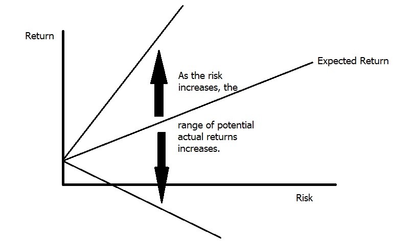
Take a few moments and think of what factors impact your level of risk aversion. Typically, we find that age, personality, number of dependents, wealth, income, variability of income, past life experiences, and other factors all combine to influence one's level of risk aversion. One last thought -- remember that taking stock D does not mean you will earn a higher return, just that you will earn a higher return on average. If you always earned a higher return from stock D, then it wouldn't be riskier. Visually, you can think of it along the lines of the diagram below. At low levels of risk, the range of returns will be close to the expected return. At high levels of risk, the range of returns will be higher. The expected return increases with risk, but so too does the range of potential returns.
Diversifiable and Non-Diversifiable Risk
Remember earlier, we discussed the possibility of lowering our firm-specific risk by holding a number of stocks from a wide range of industries? This concept of diversification allows us to greatly reduce our risk by holding a portfolio. Diversifiable risk refers to risk factors that are isolated to one particular firm or industry.
For example, if a drug manufacturer gets hit with a lawsuit related to one of the drugs it produces, that is likely to have an isolated impact. It will not have any effect on the stock prices of auto manufacturers, grocery retailers, banks, etc. Once we have enough stocks in our portfolio, bad news for any one of them will have a small impact on our overall portfolio as long as that bad news is contained to that one firm (in other words, as long as it comes from a diversifiable risk factor). By holding approximately [latex]25-50[/latex] stocks, we can eliminate a large portion of our diversifiable risk (Statman, 1987). While a portfolio of [latex]10[/latex] stocks has much less risk than a portfolio of [latex]5[/latex] stocks, a portfolio of [latex]100[/latex] stocks offers very little risk reduction compared to a much smaller 50-stock portfolio (assuming our stocks are from a variety of different industries and have other differing characteristics).
Does this mean that we have eliminated all of our risk when we hold a 50-stock (or even 500-stock) portfolio? No, we are still subject to general economic risk that affects all securities. This leftover risk is referred to as Non-diversifiable risk (or market/systematic risk). Examples of non-diversifiable risks include political events (such as wars), energy price shocks, changes in interest rates, recessions, etc. Any risk factor that impacts virtually all stocks is referred to as a non-diversifiable risk factor because it will impact our portfolio regardless of how well we have diversified our investments. Another name for non-diversifiable risk is market risk because these sources of risk tend to affect the entire market as opposed to an individual security or industry. Note: Market risk does not refer to risk impacting a specific industry. Instead, it refers to risk impacting the broad economy (most stocks). If a risk factor only impacts one or two industries without carrying over to the broader market, it is classified as firm-specific.
The following graph (Figure 9.4.2) does a good job of illustrating the concept of diversification and firm-specific vs. market risk.

Given the relative ease with which investors can virtually eliminate their firm-specific (diversifiable) risk, for most investors the level of non-diversifiable (market) risk associated with an investment becomes more important. It is important to note that while market risk impacts all stocks, it does not impact all stocks equally. Therefore, we need to a tool to measure how sensitive a stock is to the overall market. This tool is known as BETA. Standard deviation measures total risk (diversifiable risk + market risk) for a security, while beta measures the degree of market (non-diversifiable) risk. We won’t introduce a risk measurement for diversifiable risk.
Video: "Diversification" by Kevin Bracker [8:45] is licensed under the Standard YouTube License.Transcript and closed captions available on YouTube.
Attribution
"Chapter 7 - Risk Analysis" from Business Finance Essentials by Dr. Kevin Bracker; Dr. Fang Lin; and Jennifer Pursley is licensed under a Creative Commons Attribution-NonCommercial 4.0 International License, except where otherwise noted.
