8.3 Review Exercises

1. A vacation resort rents SCUBA equipment to certified divers. The resort charges an up-front fee of $25 and another fee of $12.50 an hour.

1. What are the dependent and independent variables?
2. Find the equation that expresses the total fee in terms of the number of hours the equipment is rented.
3. Graph the equation from 2.

Solution

a. dependent variable: fee amount; independent variable: time

b. [latex]y=25+12.50x[/latex]

c.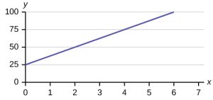

 

2. Which of the following equations are linear?

1. [latex]y = 6x + 8[/latex]
2. [latex]y + 7 = 3x[/latex]
3. [latex]y – x = 8x^2[/latex]
4. [latex]4y= 8[/latex]

Solution

a. linear

b. linear

c. not linear

d. not linear

 

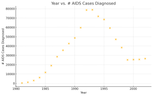
4. The table below contains real data for the first two decades of AIDS reporting.  Use the columns “year” and “# AIDS cases diagnosed. Why is “year” the independent variable and “# AIDS cases diagnosed.” the dependent variable (instead of the reverse)?

Adults and Adolescents only, United States

Year	# AIDS cases diagnosed	# AIDS deaths
Pre-1981	91	29
1981	319	121
1982	1,170	453
1983	3,076	1,482
1984	6,240	3,466
1985	11,776	6,878
1986	19,032	11,987
1987	28,564	16,162
1988	35,447	20,868
1989	42,674	27,591
1990	48,634	31,335
1991	59,660	36,560
1992	78,530	41,055
1993	78,834	44,730
1994	71,874	49,095
1995	68,505	49,456
1996	59,347	38,510
1997	47,149	20,736
1998	38,393	19,005
1999	25,174	18,454
2000	25,522	17,347
2001	25,643	17,402
2002	26,464	16,371
Total	802,118	489,093

Solution

The number of cases depends on the year. Therefore, the year becomes the independent variable, and the number of flu cases is the dependent variable.

 

5. A specialty cleaning company charges an equipment fee and an hourly labour fee. A linear equation that expresses the total amount of the fee the company charges for each session is [latex]y = 50 + 100x[/latex].

1. What are the independent and dependent variables?
2. What is the y-intercept and what is the slope? Interpret them using complete sentences.

Solution

a. independent: hour; dependent: fee.

b. The y-intercept is 50 (a = 50). At the start of the cleaning, the company charges a one-time fee of $50 (this is when x = 0). The slope is 100 (b = 100). For each session, the company charges $100 for each hour they clean.

 

6. Due to erosion, a river shoreline is losing several thousand pounds of soil each year. A linear equation that expresses the total amount of soil lost per year is [latex]y = 12,000x[/latex].

1. What are the independent and dependent variables?
2. How many pounds of soil does the shoreline lose in a year?
3. What is the y-intercept? Interpret its meaning.

Solution

a. independent: years; dependent lost soil.

b. 12,000 pounds of soil

c. y-intercept is zero means when the time (years) is zero, the loss of soil is zero.

 

7. The price of a single issue of stock can fluctuate throughout the day. A linear equation that represents the price of stock for Shipment Express is [latex]y = 15 – 1.5x[/latex] where [latex]x[/latex] is the number of hours passed in an eight-hour day of trading.

1. What are the slope and y-intercept? Interpret their meaning.
2. If you owned this stock, would you want a positive or negative slope? Why?

Solution

a. The slope is –1.5 (b = –1.5). This means the stock is losing value at a rate of $1.50 per hour. The y-intercept is $15 (a = 15). This means the price of stock before the trading day was $15.

b. A positive slope so that the stock gains value.

 

8. For each of the following situations, state the independent variable and the dependent variable.

1. A study is done to determine if elderly drivers are involved in more motor vehicle fatalities than other drivers. The number of fatalities per 100,000 drivers is compared to the age of drivers.
2. A study is done to determine if the weekly grocery bill changes based on the number of family members.
3. Insurance companies base life insurance premiums partially on the age of the applicant.
4. Utility bills vary according to power consumption.
5. A study is done to determine if a higher education reduces the crime rate in a population.

Solution

a. Independent Variable: Age of drivers
Dependent Variable: Number of fatalities per 100,000 drivers

b. Independent Variable: Number of family members
Dependent Variable: Weekly grocery bill

c. Independent Variable: Age of the applicant
Dependent Variable: Life insurance premiums

d. Independent Variable: Power consumption
Dependent Variable: Utility bills

e. Independent Variable: Level of education in the population
Dependent Variable: Crime rate in the population

 

9. Does the scatter plot appear linear? Strong, moderate, or weak? Positive or negative?

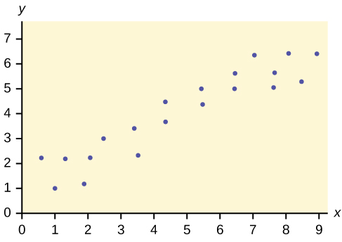
Image Description

This image is a scatter plot with the x-axis labelled as “x” and the y-axis labelled as “y.” Both axes have values ranging from 0 to 9. The background of the plot area is light yellow. There are 20 blue dots plotted, representing data points, that display a positive linear trend. As the values of x increase, the values of y tend to increase accordingly.

Solution

The plot is not linear, but it is strongly positively correlated.

 

10. Does the scatter plot appear linear? Strong, moderate, or weak? Positive or negative?

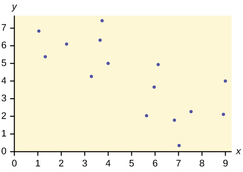
Image Description

The image is a scatter plot with a yellow background. The x-axis is labelled “x” and runs from 0 to 9, while the y-axis is labelled “y” and runs from 0 to 7. The plot features several blue dots representing data points scattered throughout the graph. The distribution of points suggests a general negative correlation between the x and y variables, as the y-values tend to decrease as the x-values increase.

Solution

The data appears to be linear with a moderate negative correlation.

 

11. Does the scatter plot appear linear? Strong, moderate, or weak? Positive or negative?

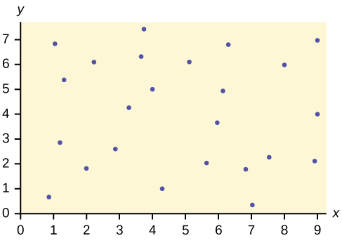
Image Description

The image is a scatter plot on a yellow background with dots that represent data points. The x-axis is labelled from 0 to 9, while the y-axis is labelled from 0 to 7. The data points are scattered across the plot area with no clear pattern or trend.

Solution

Not linear but moderately negatively correlated.

 

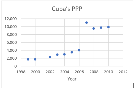
12. The Gross Domestic Product Purchasing Power Parity is an indication of a country’s currency value compared to another country. The table below shows the GDP PPP of Cuba as compared to US dollars. Construct a scatter plot of the data.

Year	Cuba’s PPP	Year	Cuba’s PPP
1999	1,700	2006	4,000
2000	1,700	2007	11,000
2002	2,300	2008	9,500
2003	2,900	2009	9,700
2004	3,000	2010	9,900
2005	3,500

Solution

 

13. Does the higher cost of tuition translate into higher-paying jobs? The table lists the top ten colleges based on mid-career salary and the associated yearly tuition costs. Construct a scatter plot of the data.

School	Mid-Career Salary (in thousands)	Yearly Tuition
Princeton	137	28,540
Harvey Mudd	135	40,133
CalTech	127	39,900
US Naval Academy	122	0
West Point	120	0
MIT	118	42,050
Lehigh University	118	43,220
NYU-Poly	117	39,565
Babson College	117	40,400
Stanford	114	54,506

Solution

 

14. A random sample of ten professional athletes produced the following data where [latex]x[/latex] is the number of endorsements the player has and [latex]y[/latex] is the amount of money made (in millions of dollars).

[latex]x[/latex]	[latex]y[/latex]	[latex]x[/latex]	[latex]y[/latex]
0	2	5	12
3	8	4	9
2	7	3	9
1	3	0	3
5	13	4	10

1. Draw a scatter plot of the data.
2. Use regression to find the equation for the line of best fit.
3. What is the slope of the line of best fit? What does it represent?
4. What is the [latex]y[/latex]-intercept of the line of best fit?
   

Solution

a.

b. [latex]ŷ = 2.23 + 1.99x[/latex]

c. The slope is 1.99 (b = 1.99). It means that for every endorsement deal a professional player gets, he gets an average of another $1.99 million in pay each year.

d. The y-intercept is 2.23.

 

15. What does an r value of zero mean?

Solution

It means that there is no correlation between the data sets.

 

16. What is the process through which we can calculate a line that goes through a scatter plot with a linear pattern?

Solution

The process through a line that goes through a scatter plot with a linear pattern is linear regression.

 

17. Explain what it means when a correlation has an [latex]r^2[/latex] of 0.72.

Solution

It means that 72% of the variation in the dependent variable (y) can be explained by the variation in the independent variable (x).

 

18. An electronics retailer used regression to find a simple model to predict sales growth in the first quarter of the new year (January through March). The model is good for 90 days, where [latex]x[/latex] is the day. The model can be written as [latex]\hat{y} = 101.32 + 2.48x[/latex] where [latex]\hat{y}[/latex] is in thousands of dollars.

1. What would you predict the sales to be on day 60?
2. What would you predict the sales to be on day 90?

Solution

a. $250,120

b. $324,520

 

19.  A landscaping company is hired to mow the grass for several large properties. The total area of the properties combined is 1,345 acres. The rate at which one person can mow is [latex]\hat{y}= 1350 – 1.2x[/latex] where [latex]x[/latex] is the number of hours and [latex]\hat{y}[/latex] represents the number of acres left to mow.

1. How many acres will be left to mow after 20 hours of work?
2. How many acres will be left to mow after 100 hours of work?
3. How many hours will it take to mow all of the lawns?

Solution

a. 1,326 acres

b. 1,230 acres

c. 1,125 hours, or when x = 1,125

 

20. The table below contains real data for the first two decades of AIDS reporting.

Adults and Adolescents only, United States

Year	# AIDS cases diagnosed	# AIDS deaths
Pre-1981	91	29
1981	319	121
1982	1,170	453
1983	3,076	1,482
1984	6,240	3,466
1985	11,776	6,878
1986	19,032	11,987
1987	28,564	16,162
1988	35,447	20,868
1989	42,674	27,591
1990	48,634	31,335
1991	59,660	36,560
1992	78,530	41,055
1993	78,834	44,730
1994	71,874	49,095
1995	68,505	49,456
1996	59,347	38,510
1997	47,149	20,736
1998	38,393	19,005
1999	25,174	18,454
2000	25,522	17,347
2001	25,643	17,402
2002	26,464	16,371
Total	802,118	489,093

1. Graph “year” versus “# AIDS cases diagnosed” (plot the scatter plot). Do not include pre-1981 data.
2. Calculate the correlation coefficient.
3. Interpret the correlation coefficient.
4. Find the linear regression equation.
5. Interpret the slope of the linear regression equation.
6. What is the predicted number of diagnosed cases for the year 1985?
7. What is the predicted number of diagnosed cases for the year 1970?  Why doesn’t this answer make sense?
8. Calculate the coefficient of determination.
9. Interpret the coefficient of determination.
10. Calculate the standard error of the estimate.
11. Interpret the standard error of the estimate.

Solution

a.

b. 0.45

c. There is a moderate positive correlation between the year and the number of AIDS cases diagnosed, indicating that, on average, AIDS cases tended to increase with time over this period, although the relationship is not very strong.

d. [latex]y=1749.78x−3448225.05y=1749.78x−3448225.05[/latex]

e. or each additional year, the number of diagnosed AIDS cases is expected to increase by approximately 1,750 cases, according to the model.

f. 25,082

g. -1,164. This prediction doesn’t make sense because the value is negative, which isn’t possible for case counts. This shows that the linear model isn’t suitable for predicting years far outside the observed range.

h. 0.20

i. Approximately 20% of the variance in the number of AIDS cases diagnosed can be explained by the year, indicating a weak fit of the linear model to the data.

j. 21,869.27

k. The standard deviation of the residuals (errors) is around 21,869 cases, indicating that the model’s predictions can differ from the actual number of cases by a substantial margin, reflecting the variability in the data that the model doesn’t capture.

 

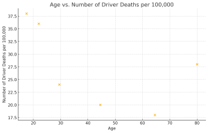
21. Recently, the annual number of driver deaths per 100,000 for the selected age groups was as follows:

Age	Number of Driver Deaths per 100,000
17.5	38
22	36
29.5	24
44.5	20
64.5	18
80	28

1. Using “ages” as the independent variable and “Number of driver deaths per 100,000” as the dependent variable, make a scatter plot of the data.
2. Calculate the least squares (best–fit) line.
3. Interpret the slope of the least squares line.
4. Predict the number of deaths of people aged 40.
5. Find the correlation coefficient.
6. Interpret the correlation coefficient.
7. Find the coefficient of determination.
8. Interpret the coefficient of determination.
9. Find the standard error of the estimate.
10. Interpret the standard error of the estimate.

Solution

a.

b. [latex]y=−0.19x+35.58y=−0.19x+35.58[/latex]

c. The slope of -0.19 indicates that, on average, the number of driver deaths per 100,000 decreases by about 0.19 for each additional year of age.

d. Approximately 27.91 deaths per 100,000.

e. -0.58

f. There is a moderate negative correlation between age and the number of driver deaths per 100,000, meaning that as age increases, the number of driver deaths tends to decrease to some extent.

g. 0.33

h. About 33% of the variance in the number of driver deaths per 100,000 can be explained by age, which indicates a moderate fit of the linear model to the data.

i. 6.15

j. The standard deviation of the residuals (errors) is approximately 6.15 deaths per 100,000, which means that predictions based on this model can deviate from actual values by about 6.15 on average, reflecting the spread of the data around the regression line.

 

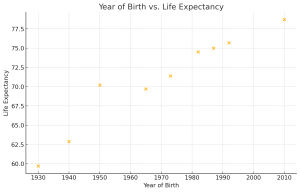
22. The table below shows the life expectancy for an individual born in the United States in certain years.

Year of Birth	Life Expectancy
1930	59.7
1940	62.9
1950	70.2
1965	69.7
1973	71.4
1982	74.5
1987	75
1992	75.7
2010	78.7

1. Decide which variable should be the independent variable and which should be the dependent variable.
2. Draw a scatter plot of the ordered pairs.
3. Find the correlation coefficient
4. Interpret the correlation coefficient.
5. Find the linear regression equation.
6. Interpret the slope of the linear regression equation.
7. What is the estimated life expectancy for someone born in 1950?  Why doesn’t this value match the life expectancy given in the table for 1950?
8. What is the estimated life expectancy for someone born in 1982?
9. Using the regression equation, find the estimated life expectancy for someone born in 1850.  Is this an accurate estimate for that year?  Explain why or why not.
10. Calculate the coefficient of determination.
11. Interpret the coefficient of determination.
12. Calculate the standard error of the estimate.
13. Interpret the standard error of the estimate.

Solution

a. Independent Variable: Year of Birth
Dependent Variable: Life Expectancy

b.

c. 0.96

d. There is a strong positive correlation between the year of birth and life expectancy, suggesting that life expectancy has generally increased over time.

e. [latex]y=0.23x−377.24y=0.23x−377.24[/latex]

f. The slope of 0.23 means that for each additional year, the life expectancy increases by approximately 0.23 years.

g. 66.34 years. This estimate does not match the actual life expectancy given in the table (70.2 years) because the linear regression equation provides an average trend, not exact values for each year.

h. 73.62 years

i. 43.59 years. This estimate is not accurate for that year because the regression model is based on data from 1930 onward. Extrapolating back to 1850 goes beyond the data’s range, where the trend may not apply.

j. 0.92

k. Approximately 92% of the variance in life expectancy can be explained by the year of birth, indicating a very strong fit of the model to the data.

l. 1.61

m. The standard deviation of the residuals (errors) is approximately 1.61 years, indicating that predicted life expectancy values typically differ from actual values by about 1.61 years.

 

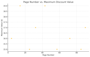
23. The maximum discount value of the Entertainment® card for the “Fine Dining” section, Edition ten, for various pages is given in the table below.

Page number	Maximum value ($)
4	16
14	19
25	15
32	17
43	19
57	15
72	16
85	15
90	17

1. Decide which variable should be the independent variable and which should be the dependent variable.
2. Draw a scatter plot of the ordered pairs.
3. Find the correlation coefficient.
4. Interpret the correlation coefficient.
5. Find the linear regression equation.
6. Interpret the slope of the linear regression equation.
7. What is the estimated maximum value for restaurants on page 10?
8. What is the estimated maximum value for restaurants on page 70?
9. Using the regression equation, find the estimated maximum value for restaurants on page 200.  Is this an accurate estimate for that page?  Explain why or why not.
10. Calculate the coefficient of determination.
11. Interpret the coefficient of determination.
12. Calculate the standard error of the estimate.
13. Interpret the standard error of the estimate.

Solution

a. Independent Variable: Page Number
Dependent Variable: Maximum Discount Value

b.

c. -0.28

d. There is a weak negative correlation between page number and maximum discount value, suggesting a slight tendency for the maximum value to decrease as the page number increases, though the relationship is weak.

e. [latex]y=−0.01x+17.22y=−0.01x+17.22[/latex]

f. The slope of -0.01 indicates that, on average, the maximum discount value decreases by about 1 cent for each additional page number.

g.  Approximately $17.08

h. Approximately $16.23

i. Approximately $14.39. This estimate may not be accurate for page 200 because it is far outside the range of observed page numbers, and the trend seen in the available data may not hold at such a high page number.

j. 0.08

k. Only about 8% of the variance in the maximum discount value can be explained by the page number, indicating a very weak fit of the linear model to the data.

l. 1.44

m. The standard deviation of the residuals is about $1.44, suggesting that predictions from this model may differ from actual values by around $1.44, which is relatively high given the small range of discount values.

 

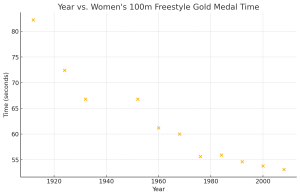
24. The table below gives the gold medal times for every other Summer Olympics for the women’s 100-meter freestyle (swimming).

Year	Time (seconds)
1912	82.2
1924	72.4
1932	66.8
1952	66.8
1960	61.2
1968	60.0
1976	55.65
1984	55.92
1992	54.64
2000	53.8
2008	53.1

1. Decide which variable should be the independent variable and which should be the dependent variable.
2. Draw a scatter plot of the ordered pairs.
3. Find the correlation coefficient.
4. Interpret the correlation coefficient.
5. Find the linear regression equation.
6. Interpret the slope of the linear regression equation.
7. What is the estimated gold medal time for 1932?
8. What is the estimated gold medal time for 1984?
9. Calculate the coefficient of determination.
10. Interpret the coefficient of determination.
11. Calculate the standard error of the estimate.
12. Interpret the standard error of the estimate.

Solution

a. Independent Variable: Year
Dependent Variable: Time (in seconds)

b.

c. -0.95

d. There is a strong negative correlation between the year and the gold medal time, indicating that as time progressed, the gold medal time generally decreased.

e. [latex]y=−0.28x+603.43y=−0.28x+603.43[/latex]

f. The slope of -0.28 suggests that, on average, the gold medal time decreased by approximately 0.28 seconds for each additional year.

g. Approximately 70.97 seconds

h. Approximately 56.63 seconds

i. 0.90

j. About 90% of the variance in gold medal times can be explained by the year, indicating that the model provides a strong fit to the data.

k. 2.70 seconds

l. The standard deviation of the residuals is approximately 2.70 seconds, suggesting that predictions from this model typically differ from actual values by about 2.70 seconds, reflecting a reasonably good fit of the linear trend to the data. ​

​
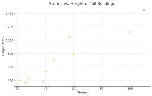
25. The height (sidewalk to roof) of notable tall buildings in America is compared to the number of stories of the building (beginning at street level).

Height (in feet)	Stories
1,050	57
428	28
362	26
529	40
790	60
401	22
380	38
1,454	110
1,127	100
700	46

1. Using “stories” as the independent variable and “height” as the dependent variable, draw a scatter plot of the ordered pairs.
2. Find the correlation coefficient.
3. Interpret the correlation coefficient.
4. Find the linear regression equation.
5. Interpret the slope of the linear regression equation.
6. What is the estimated height for a 32-story building?
7. What is the estimated height for a 94-story building?
8. Using the regression equation, find the estimated height for a 6-story building.  Is this an accurate estimate for the height of a 6-story building?  Explain why or why not.
9. Calculate the coefficient of determination.
10. Interpret the coefficient of determination.
11. Calculate the standard error of the estimate.
12. Interpret the standard error of the estimate.

Solution

a.

b. 0.94

c. There is a strong positive correlation between the number of stories and building height, indicating that taller buildings generally have more stories.

d. [latex]y=11.76x+102.43y=11.76x+102.43[/latex]

e. The slope of 11.76 suggests that, on average, each additional story adds approximately 11.76 feet to the building’s height.

f. Approximately 478.70 feet

g. Approximately 1207.72 feet

h. Approximately 172.98 feet. This estimate might not be accurate for a 6-story building as it lies outside the typical range of the dataset (mainly taller buildings), so the trend may not apply well for such a small number of stories.

i. 0.89

j. Approximately 89% of the variance in building height can be explained by the number of stories, indicating that the linear model provides a strong fit to the data.

k. 118.75 feet

l. The standard deviation of the residuals is approximately 118.75 feet, indicating that predictions from this model can typically differ from actual values by around 118.75 feet, which suggests some variability in the height-to-story relationship across the buildings.

 

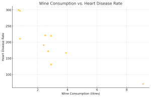
26. The following table shows data on average per capita wine consumption and heart disease rate in a random sample of 10 countries.

Yearly wine consumption in litres	2.5	3.9	2.9	2.4	2.9	0.8	9.1	2.7	0.8	0.7
Death from heart diseases	221	167	131	191	220	297	71	172	211	300

1. Decide which variable should be the independent variable and which should be the dependent variable.
2. Draw a scatter plot of the ordered pairs.
3. Find the correlation coefficient.
4. Interpret the correlation coefficient.
5. Find the linear regression equation.
6. Interpret the slope of the linear regression equation.
7. Calculate the coefficient of determination.
8. Interpret the coefficient of determination.
9. Calculate the standard error of the estimate.
10. Interpret the standard error of the estimate.

Solution

a. Independent Variable: Yearly Wine Consumption (litres)
Dependent Variable: Heart Disease Rate

b.

c. -0.84

d. There is a strong negative correlation between wine consumption and heart disease rate, suggesting that, as average wine consumption increases, the heart disease rate tends to decrease.

e. [latex]y=−23.88x+266.63y=−23.88x+266.63[/latex]

f. The slope of -23.88 suggests that, on average, for each additional litre of wine consumed per capita, the heart disease rate decreases by approximately 23.88 deaths per 100,000.

g. 0.70

h. About 70% of the variance in heart disease rates can be explained by wine consumption, indicating that the linear model provides a reasonably strong fit to the data.

i. 36.28

j. The standard deviation of the residuals (errors) is approximately 36.28 deaths per 100,000, meaning that predictions from this model typically differ from actual values by about 36.28, reflecting a moderate level of variability around the regression line. ​

 

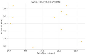
27. The following table consists of one student athlete’s time (in minutes) to swim 2000 yards and the student’s heart rate (beats per minute) after swimming on a random sample of 10 days:

Swim Time	Heart Rate
34.12	144
35.72	152
34.72	124
34.05	140
34.13	152
35.73	146
36.17	128
35.57	136
35.37	144
35.57	148

1. Decide which variable should be the independent variable and which should be the dependent variable.
2. Draw a scatter plot of the ordered pairs.
3. Find the correlation coefficient.
4. Interpret the correlation coefficient.
5. Find the linear regression equation.
6. Interpret the slope of the linear regression equation.
7. What is the estimated heart rate for a swim time of 34.75 minutes?
8. Calculate the coefficient of determination.
9. Interpret the coefficient of determination.
10. Calculate the standard error of the estimate.
11. Interpret the standard error of the estimate.

Solution

a. Independent Variable: Swim Time (minutes)
Dependent Variable: Heart Rate (BPM)

b.

c. -0.12

d. There is a very weak negative correlation between swim time and heart rate, suggesting almost no relationship between the two variables.

e. [latex]y=−1.49x+193.88y=−1.49x+193.88[/latex]

f. The slope of -1.49 suggests that, on average, each additional minute of swim time slightly decreases the heart rate by about 1.49 BPM, though this effect is minimal.

g. Approximately 141.95 BPM

h. 0.02

i. Only about 2% of the variance in heart rate can be explained by swim time, indicating that the linear model does not effectively describe the data.

j. 8.97 BPM

k. The standard deviation of the residuals (errors) is approximately 8.97 BPM, indicating that predictions from this model typically differ from actual values by around 8.97 BPM, reflecting the weak relationship and poor predictive accuracy of the model. ​

 

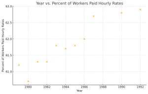
28. The table below gives percent of workers who are paid hourly rates for the years 1979 to 1992.

Year	Percent of workers paid hourly rates
1979	61.2
1980	60.7
1981	61.3
1982	61.3
1983	61.8
1984	61.7
1985	61.8
1986	62.0
1987	62.7
1990	62.8
1992	62.9

1. Decide which variable should be the independent variable and which should be the dependent variable.
2. Draw a scatter plot of the ordered pairs.
3. Find the correlation coefficient.
4. Interpret the correlation coefficient.
5. Find the linear regression equation.
6. Interpret the slope of the linear regression equation.
7. What is the estimated percentage of workers paid hourly rates in 1988?
8. Calculate the coefficient of determination.
9. Interpret the coefficient of determination.
10. Calculate the standard error of the estimate.
11. Interpret the standard error of the estimate.

Solution

a. Independent Variable: Year
Dependent Variable: Percent of Workers Paid Hourly Rates

b.

c. 0.94

d. There is a strong positive correlation between the year and the percentage of workers paid hourly rates, suggesting that this percentage has generally increased over time.

e. [latex]y=0.17x−266.89y=0.17x−266.89[/latex]

f. The slope of 0.17 indicates that, on average, the percentage of workers paid hourly rates increased by about 0.17% each year.

g. Approximately 62.42%

h. 0.89

i. About 89% of the variance in the percentage of workers paid hourly rates can be explained by the year, indicating a very strong fit of the linear model to the data.

j. 0.22%

k. The standard deviation of the residuals is approximately 0.22%, meaning that predictions from this model typically differ from actual values by around 0.22%, showing a high degree of accuracy in the model’s predictions.

 

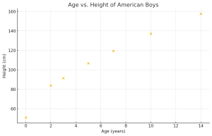
29. The table below shows the average heights for American boys in 1990.

Age (years)	Height (cm)
birth	50.8
2	83.8
3	91.4
5	106.6
7	119.3
10	137.1
14	157.5

1. Decide which variable should be the independent variable and which should be the dependent variable.
2. Draw a scatter plot of the ordered pairs.
3. Find the correlation coefficient.
4. Interpret the correlation coefficient.
5. Find the linear regression equation.
6. Interpret the slope of the linear regression equation.
7. What is the estimated average height for a one-year-old?
8. Using the regression equation, find the estimated average height for a 62-year-old man.  Do you think that your answer is reasonable?  Explain why or why not.
9. Calculate the coefficient of determination.
10. Interpret the coefficient of determination.
11. Calculate the standard error of the estimate.
12. Interpret the standard error of the estimate.

Solution

a. Independent Variable: Age (years)
Dependent Variable: Height (cm)

b.

c. 0.98

d. There is a very strong positive correlation between age and height, indicating that as age increases, height generally increases as well.

e. [latex]y=7.09x+65.09y=7.09x+65.09[/latex]

f. The slope of 7.09 indicates that, on average, height increases by about 7.09 cm for each additional year of age.

g. Approximately 72.18 cm

h. Approximately 504.97 cm. This prediction is not reasonable as it suggests an implausible height. The model is only accurate for the age range of the data (birth to 14 years), where growth patterns are different from those in adulthood. Extrapolating far beyond this range leads to unrealistic results.

i. 0.95

j. About 95% of the variance in height can be explained by age, indicating an excellent fit of the linear model to the data within the observed range.

k. 7.13 cm

l. The standard deviation of the residuals is approximately 7.13 cm, meaning predictions from this model typically differ from actual values by around 7.13 cm within the age range of the data. ​