2.1 Limits and Continuity
Introduction
Precalculus Idea: Slope and Rate of Change
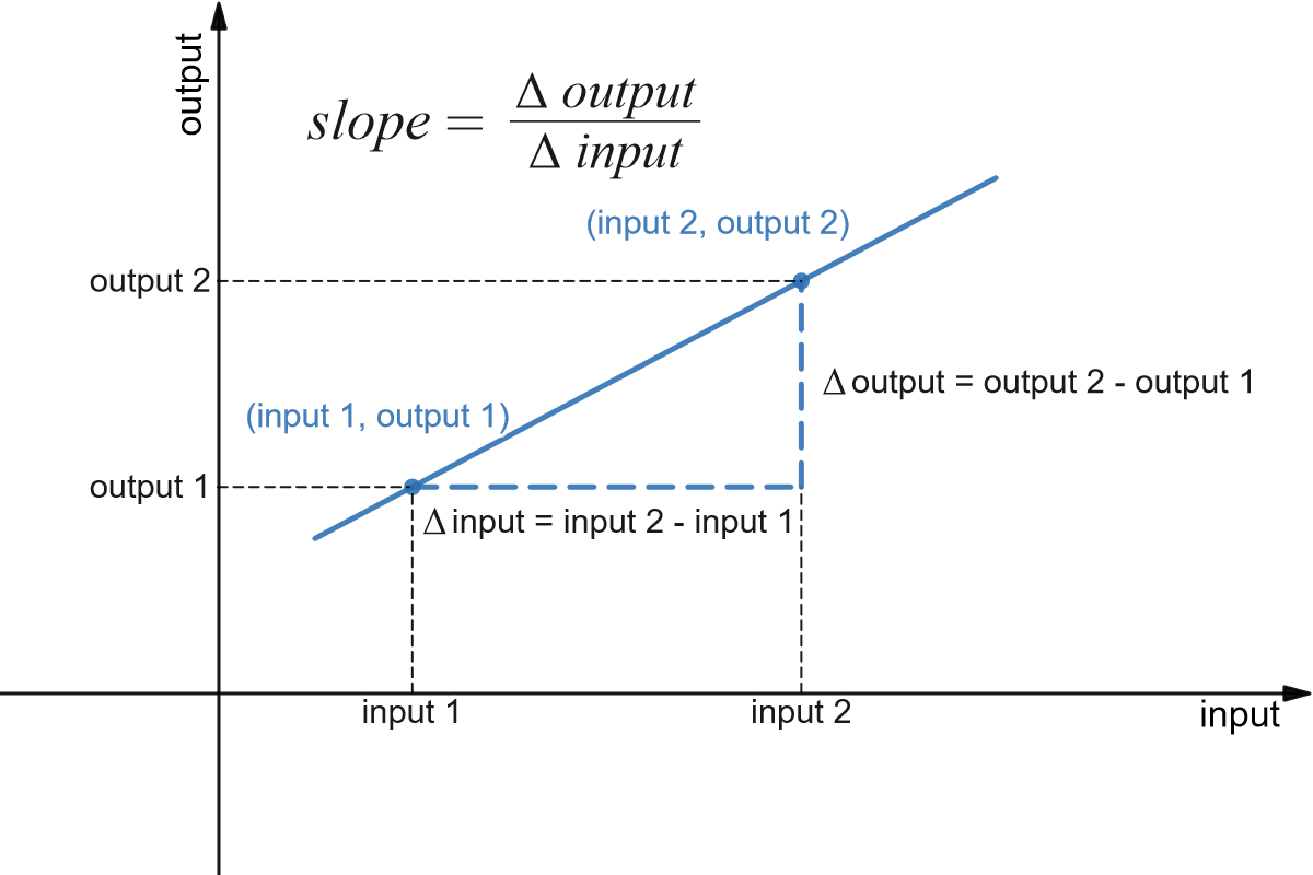
[latex]\text{slope between two points}=\dfrac{\Delta \text{output}}{\Delta \text{input}}=\dfrac{\text{output}_2-\text{output}_1}{\text{input}_2-\text{input}_1}[/latex]
We can also think of slope in contextual, not graph terms. It represents the rate of change in output in relation to the change in input. The value of slope will tell us whether the line connecting the two points is flat or going up or going down, and by how much over one horizontal unit. In the context of rate of change, this value will tell us how, and by how much, the output is changing with respect change in one unit of input.
So when we talk about slope, we are talking about slope between two points. Equivalently, when we talk about rate of change, we are talking about two input-output pairs and how the change from one to the other can be described. Therefore, we always need two pairs of input-output vales.
However, if you are walking up a hill, or walking down a hill and you stop, you'll still think of being on "a steep slope" or "a gentle slope" even though the hill you are on is not a straight line. Note that when you are thinking about the slope at the point you are standing, this is not specific to a slope between two points on the hill. So where does that sense of slope on a hill come from? It comes from approximating the steepness (and the direction, as in up or down) by brain picking two imaginary points close to where you are standing and getting a rough estimate of slope. This concept, of being able to calculate slope at a single point, without a reference to some other specific point, is fundamentally behind the concept of "instantaneous rate of change", which we will discuss throughout this chapter.
So, we would like to be able to get that same sort of information about slope (how fast the curve rises or falls, velocity from distance) even if the graph is not a straight line. But what happens if we try to find the slope of a curve, as in the figure below?
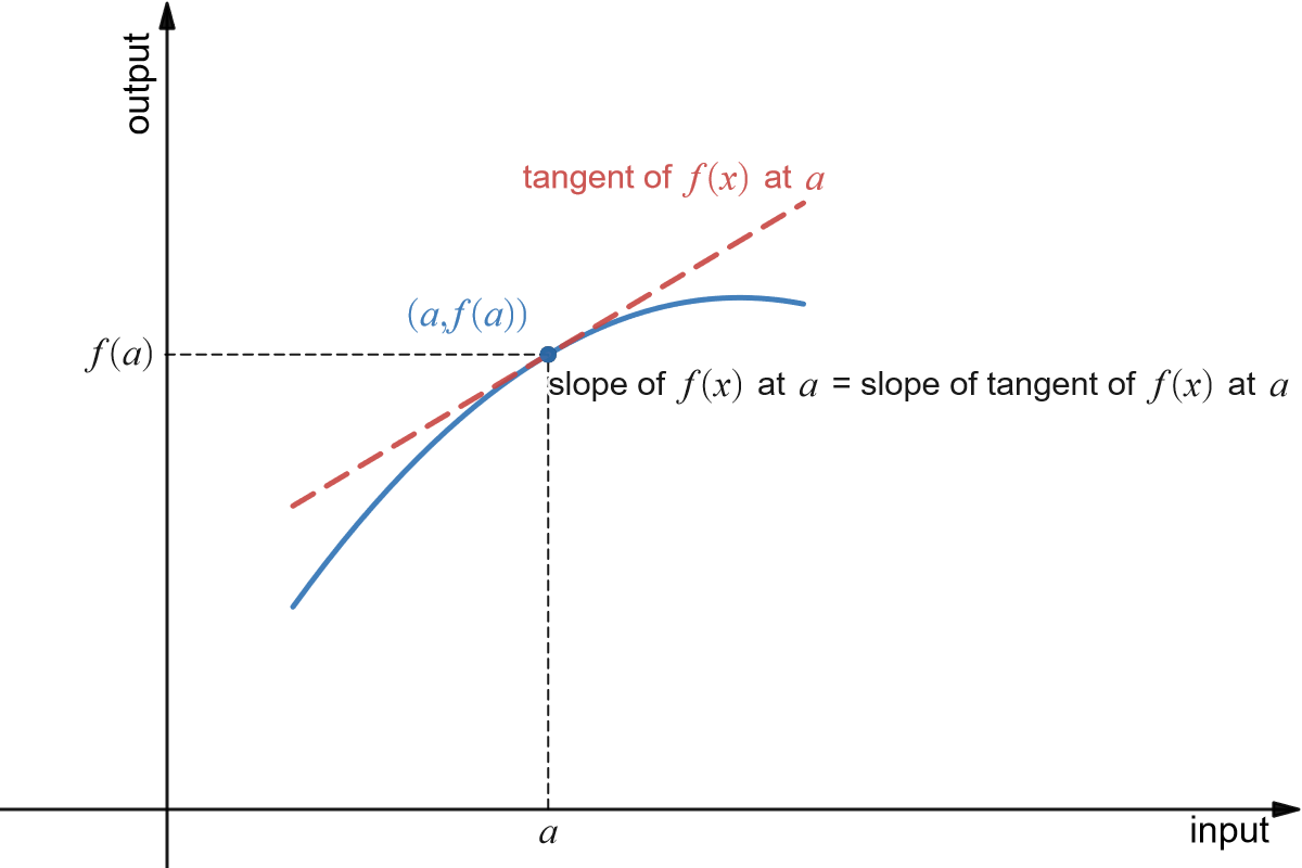 So if we need two points in order to determine the slope of a line, how can we find a slope of a curve at just one point? The answer, as suggested in the figure, is to find the slope of the tangent line to the curve at that point. Most of us have an intuitive idea of what a tangent line is. Unfortunately, “tangent line” is hard to define precisely.
Definition (Secant Line)
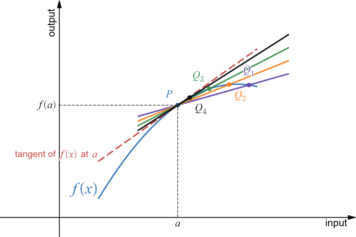
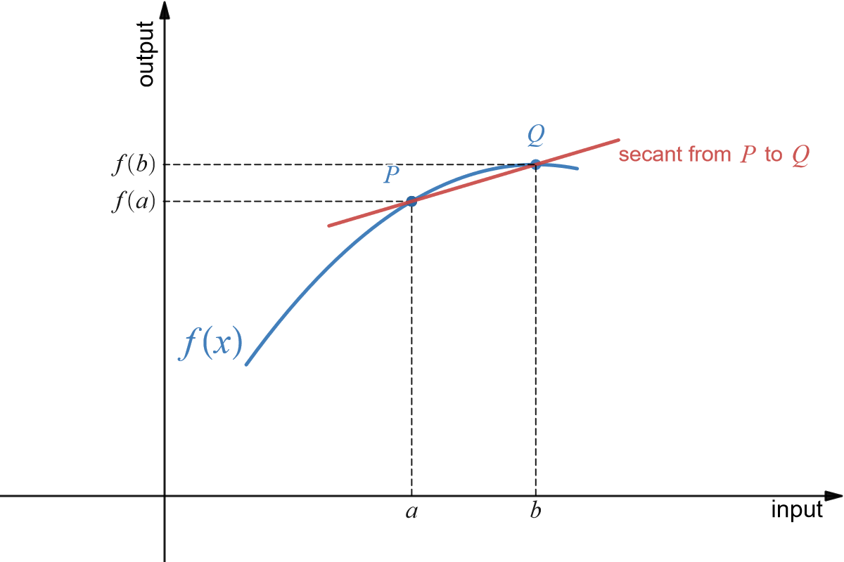 Can't-quite-do-it-yet Definition (Tangent Line)
Section 2.1: Limits and Continuity
Limits

Definition (Limit)
- [latex]f(c)[/latex] is a single number that describes the behavior (value) of [latex]f(x)[/latex] at the point [latex]x = c[/latex].
- [latex]\lim\limits_{x\to c} f(x)[/latex] is a single number that describes the behavior of [latex]f(x)[/latex] near, but NOT at , the point [latex]x = c[/latex].
Example 1
- [latex]\lim\limits_{x\to 1} f(x)[/latex]
- [latex]\lim\limits_{x\to 2} f(x)[/latex]
- [latex]\lim\limits_{x\to 3} f(x)[/latex]
- [latex]\lim\limits_{x\to 4} f(x)[/latex]
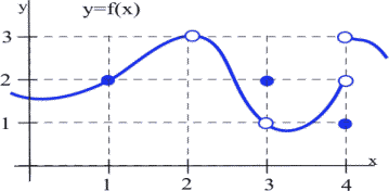
- When [latex]x[/latex] is very close to 1, the values of [latex]f(x)[/latex] are very close to [latex]y = 2[/latex]. In this example, it happens that [latex]f(1) = 2[/latex], but that is irrelevant for the limit. The only thing that matters is what happens for [latex]x[/latex] close to 1 but [latex]x \neq 1[/latex].
- [latex]f(2)[/latex] is undefined, but we only care about the behavior of [latex]f(x)[/latex] for [latex]x[/latex] close to 2 but not equal to 2. When [latex]x[/latex] is close to 2, the values of [latex]f(x)[/latex] are close to 3. If we restrict [latex]x[/latex] close enough to 2, the values of [latex]y[/latex] will be as close to 3 as we want, so [latex]\lim\limits_{x\to 2} f(x) = 3[/latex].
- When [latex]x[/latex] is close to 3 (or "as [latex]x[/latex] approaches the value 3"), the values of [latex]f(x)[/latex] are close to 1 (or "approach the value 1"), so [latex]\lim\limits_{x\to 3} f(x) = 1[/latex]. For this limit it is completely irrelevant that [latex]f(3) = 2[/latex], We only care about what happens to [latex]f(x)[/latex] for [latex]x[/latex] close to and not equal to 3.
- This one is harder and we need to be careful. When [latex]x[/latex] is close to 4 and slightly less than 4 ([latex]x[/latex] is just to the left of 4 on the [latex]x[/latex]-axis), then the values of [latex]f(x)[/latex] are close to 2. But if [latex]x[/latex] is close to 4 and slightly larger than 4 then the values of [latex]f(x)[/latex] are close to 3. If we only know that [latex]x[/latex] is very close to 4, then we cannot say whether [latex]y = f(x)[/latex] will be close to 2 or close to 3–it depends on whether [latex]x[/latex] is on the right or the left side of 4. In this situation, the [latex]f(x)[/latex] values are not close to a single number so we say [latex]f(x)[/latex] does not exist. It is irrelevant that [latex]f(4) = 1[/latex]. The limit, as [latex]x[/latex] approaches 4, would still be undefined if [latex]f(4)[/latex] was 3 or 2 or anything else.
We can also explore limits using tables and using algebra: view video example.
(by Eric Bancroft, licensed under a Creative Commons Attribution-NonCommercial-NoDerivatives 4.0 International License)
Example 2
Answer:
You might try to evaluate at [latex]x = 1[/latex], but [latex]f(x)[/latex] is not defined at [latex]x = 1[/latex]. It is tempting, but incorrect , to conclude that this function does not have a limit as [latex]x[/latex] approaches 1.
| [latex]x[/latex] | [latex]f(x)[/latex] |
| 0.9 | 2.82 |
| 0.9998 | 2.9996 |
| 0.999994 | 2.999988 |
| 0.9999999 | 2.9999998 |
| $latex \to 1 $ | $latex \to 3 $ |
| [latex]x[/latex] | [latex]f(x)[/latex] |
| 1.1 | 3.2 |
| 1.003 | 3.006 |
| 1.0001 | 3.0002 |
| 1.000007 | 3.000014 |
| [latex]\to 1[/latex] | [latex]\to 3[/latex] |
The function [latex]f[/latex] is not defined at [latex]x = 1[/latex], but when [latex]x[/latex] is close to 1, the values of [latex]f(x)[/latex] are getting very close to 3. We can get [latex]f(x)[/latex] as close to 3 as we want by taking [latex]x[/latex] very close to 1 so \[\lim\limits_{x\to 1} \dfrac{2x^2-x-1}{x-1}=3.\]

Example 3
Answer:
Notice that this function is not defined at [latex]x = 3[/latex]. We can find the limit using algebra. Giving the two terms in the numerator a common denominator, we can simplify:
View video of another example.
(by Eric Bancroft, licensed under a Creative Commons Attribution-NonCommercial-NoDerivatives 4.0 International License)
One Sided Limits
Definition (Left and Right Limits)
Example 4

See the analysis of limits through a video of another example.
(by Eric Bancroft, licensed under a Creative Commons Attribution-NonCommercial-NoDerivatives 4.0 International License)
Continuity
Definition (Continuity at a Point)
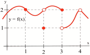
| [latex]a[/latex] | [latex]f(a)[/latex] | [latex]\lim\limits_{x\to a} f(x)[/latex] |
| 1 | 2 | 2 |
| 2 | 1 | 2 |
| 3 | 2 | Does not exist (DNE) |
| 4 | Undefined | 2 |
Review video: Continuity
(by Eric Bancroft, licensed under a Creative Commons Attribution-NonCommercial-NoDerivatives 4.0 International License)
Example 5
a. [latex]\lim\limits_{x\to 2} x^3-4x[/latex]
b. [latex]\lim\limits_{x\to 2} \dfrac{x-4}{x+3}[/latex]
c. [latex]\lim\limits_{x\to 2} \dfrac{x-4}{x-2}[/latex]
Answer:
a. The given function is polynomial, and is defined for all values of x, so we can find the limit by direct substitution:\[ \lim\limits_{x\to 2} x^3-4x = 2^3-4(2) = 0. \]
