15.3 Control Charts for Attributes
LEARNING OBJECTIVES
- Calculate the centerline, upper control limit, and lower control limit for a [latex]p[/latex]-chart or a [latex]c[/latex]-chart.
Control charts that are used to monitor the percent of defective items or the number of defects are called control charts for attributes. There are two different types of control charts for attributes—control charts for the percent defective and control charts for the number of defects. Control charts for percent defective, called [latex]p[/latex]-charts, monitor the percent of defective items in a sample. For example, if a company produces batteries, a [latex]p[/latex]-chart might be used to monitor the percent of defective batteries produced each day. Control charts for number of defects, called [latex]c[/latex]-charts, monitor the number of defects per item in a sample. For example, if a company produces lightbulbs, a [latex]c[/latex]-chart might be used to monitor the number of defects per lightbulb in a sample of lightbulbs.
[latex]p[/latex]-Charts
A [latex]p[/latex]-chart monitors the percent of defective items in a sample. To construct a [latex]p[/latex]-chart, a collection of samples, all of the same size [latex]n[/latex], are taken, the percent of defective items in each sample is calculated, and the sample proportions are plotted on the control chart. Because a [latex]p[/latex]-chart is based on samples taken from a population, [latex]p[/latex]-charts are based on the sampling distribution of the sample proportions.
Recall that the sampling distribution of the sample proportions [latex]\hat{p}[/latex] is the distribution of the sample proportions from all possible samples of size [latex]n[/latex] taken from a population. The distribution of the sample proportions follows a normal distribution if both [latex]n\times p\geq5[/latex] and [latex]n\times(1-p)\geq5[/latex]. As well,
[latex]\displaystyle{\mu_{\hat{p}}=p\;\;\;\;\;\;\;\;\;\;\sigma_{\hat{p}}=\sqrt{\frac{p\times(1-p)}{n}}}[/latex]
where [latex]\mu_{\hat{p}}[/latex] is the mean of the sample proportions, [latex]\sigma_{\hat{p}}[/latex] is the standard deviation of the sample proportions, [latex]p[/latex] is the population proportion, and [latex]n[/latex] is the sample size.
Recall that the Empirical Rule for normal distributions states that [latex]95\%[/latex] of the observations fall within two standard deviations of the mean and [latex]99.7\%[/latex] of the observations fall within three standard deviations of the mean. Assuming the [latex]n\times p\geq5[/latex] and [latex]n\times(1-p)\geq5[/latex] conditions are met, the distribution of the sample proportions follows a normal distribution. The Empirical Rule applies to the distribution of the sample proportions and implies that:
- [latex]95\%[/latex] of the sample proportions [latex]\hat{p}[/latex] fall within two standard deviations [latex]\sigma_{\hat{p}}[/latex] of the mean [latex]\mu_{\hat{p}}[/latex]. In other words, [latex]95\%[/latex] of the sample proportions fall in between the values of [latex]\mu_{\hat{p}}-2\sigma_{\hat{p}}[/latex] and [latex]\mu_{\hat{p}}+2\sigma_{\hat{p}}[/latex].
- [latex]99.7\%[/latex] of the sample proportions [latex]\hat{p}[/latex] fall within three standard deviations [latex]\sigma_{\hat{p}}[/latex] of the mean [latex]\mu_{\hat{p}}[/latex]. In other words, [latex]99.7\%[/latex] of the sample proportions fall in between the values of [latex]\mu_{\hat{p}}-3\sigma_{\hat{p}}[/latex] and [latex]\mu_{\hat{p}}+3\sigma_{\hat{p}}[/latex].
This application of the Empirical Rule to the distribution of the sample proportions forms the basis for the upper and lower control limits on a [latex]p[/latex]-chart. I the context of quality control and a [latex]p[/latex]-chart, if the sample proportion [latex]\hat{p}[/latex] falls within three standard deviations above or below the mean value, then the process is considered in-control with [latex]99.7\%[/latex] confidence. In other words, if a sample proportion falls outside the three standard deviations, then the process is out-of-control with [latex]99.7\%[/latex] confidence. Similarly, if the sample proportion [latex]\hat{p}[/latex] falls within two standard deviations above or below the mean value, then the process is considered in-control with [latex]95\%[/latex] confidence.
The centerline, the upper control limit, and the lower control limit for the [latex]p[/latex]-chart are:
[latex]\begin{eqnarray*}\text{Centerline}&=&\overline{p}\\\text{Upper Control Limit}&=&\overline{p}+z\times\sqrt{\frac{\overline{p}\times (1-\overline{p})}{n}}\\\text{Lower Control Limit}&=&\overline{p}-z\times\sqrt{\frac{\overline{p}\times (1-\overline{p})}{n}}\\\\\overline{p}&=&\text{mean proportion of the population}\\&&\text{or mean of the sample proportions}\\n&=&\text{sample size}\\z&=&\text{number of standard deviations}\\&&(2\text{ for }95\%\text{ confidence and }3\text{ for }99.7\%\text{ confidence})\end{eqnarray*}[/latex]
NOTE
The value of [latex]\overline{p}[/latex] depends on the information available. In the population proportion [latex]p[/latex] is available, then [latex]\overline{p}[/latex] is the value of [latex]p[/latex]. In many situations, the population proportion is not available. In these cases, [latex]\overline{p}[/latex] is the mean of the sample proportions.
EXAMPLE
A company manufactures batteries. In the past, the percent of defective batteries produced was [latex]2.5\%[/latex]. Suppose samples of size [latex]240[/latex] are taken. Calculate the centerline, the upper control limit, and the lower control limit for the [latex]p[/latex]-chart to monitor the percent of defect batteries at [latex]95\%[/latex] confidence.
Solution
From the question, we have [latex]\overline{p}=0.025[/latex] and [latex]n=240[/latex]. At [latex]95\%[/latex] confidence, [latex]z=2[/latex].
[latex]\begin{eqnarray*}\text{Centerline}&=&\overline{p}\\&=&0.025\\\\\text{Upper Control Limit}&=&\overline{p}+z\times\sqrt{\frac{\overline{p}\times(1-\overline{p})}{n}}\\&=&0.025+2\times\sqrt{\frac{0.025\times(1-0.025)}{240}}\\&=&0.0452\\\\\text{Lower Control Limit}&=&\overline{p}-z\times\sqrt{\frac{\overline{p}\times(1-\overline{p})}{n}}\\&=&0.025-2\times\sqrt{\frac{0.025\times(1-0.025)}{240}}\\&=&0.0048\\\end{eqnarray*}[/latex]
NOTES
- The sample proportions follow a normal distribution because [latex]n\times p=240\times 0.025=6\geq5[/latex] and [latex]n\times(1-p)=240\times(1-0.025)=234\geq5[/latex].
- Because this chart is for [latex]95\%[/latex] confidence, the value of [latex]z[/latex] in the formulas for the upper and lower control limits is [latex]2[/latex]. This sets the upper and lower control limits at [latex]2[/latex] standard deviations above and below the centerline, respectively.
- Because a [latex]p[/latex]-chart monitors percents, the centerline, the upper control limit, and the lower control limit are percents. In this example, the centerline, upper control limit, and lower control limit are [latex]2.5\%[/latex], [latex]4.52\%[/latex], and [latex]0.48\%[/latex], respectively.
EXAMPLE
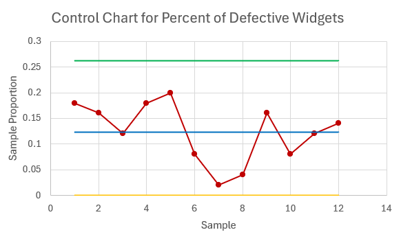
A company produces widgets. A quality control inspector monitors the percentage of defective widgets produced during the manufacturing process. For a 12-day period, the inspector takes a sample of [latex]50[/latex] widgets a day and counts the number of defective widgets in the sample. The data is recorded in the table below.
| Day | Number of Defective Widgets |
|---|---|
| 1 | 9 |
| 2 | 8 |
| 3 | 6 |
| 4 | 9 |
| 5 | 10 |
| 6 | 4 |
| 7 | 1 |
| 8 | 2 |
| 9 | 8 |
| 10 | 4 |
| 11 | 6 |
| 12 | 7 |
- Calculate the centerline, the upper control limit, and the lower control limit for the [latex]p[/latex]-chart to monitor the percent of defective widgets at [latex]99.7\%[/latex] confidence.
- Construct the [latex]p[/latex]-chart. Is the process in-control? Explain.
Solution
- From the question, we have [latex]n=50[/latex]. Because the population proportion [latex]p[/latex] is unknown, we need to calculate the mean of the sample proportions to use for [latex]\overline{p}[/latex].
Day Number of Defective Widgets Sample Proportion 1 [latex]9[/latex] [latex]0.18[/latex] 2 [latex]8[/latex] [latex]0.16[/latex] 3 [latex]6[/latex] [latex]0.12[/latex] 4 [latex]9[/latex] [latex]0.18[/latex] 5 [latex]10[/latex] [latex]0.2[/latex] 6 [latex]4[/latex] [latex]0.08[/latex] 7 [latex]1[/latex] [latex]0.02[/latex] 8 [latex]2[/latex] [latex]0.04[/latex] 9 [latex]8[/latex] [latex]0.16[/latex] 10 [latex]4[/latex] [latex]0.08[/latex] 11 [latex]6[/latex] [latex]0.12[/latex] 12 [latex]7[/latex] [latex]0.14[/latex] The mean of the sample proportions is
[latex]\begin{eqnarray*}\overline{p}&=&\frac{0.18+0.16+0.12+0.18+0.2+0.08+0.02+0.04+0.16+0.08+0.12+0.14}{12}\\&=&0.1233\ldots\end{eqnarray*}[/latex]
At [latex]99.7\%[/latex] confidence [latex]z=3[/latex].
[latex]\begin{eqnarray*}\text{Centerline}&=&\overline{p}\\&=&0.1233\\\\\text{Upper Control Limit}&=&\overline{p}+z\times\sqrt{\frac{\overline{p}\times(1-\overline{p})}{n}}\\&=&0.1233\ldots+3\times\sqrt{\frac{0.1233\ldots\times(1-0.1233\ldots)}{50}}\\&=&0.2628\\\\\text{Lower Control Limit}&=&\overline{p}-z\times\sqrt{\frac{\overline{p}\times(1-\overline{p})}{n}}\\&=&0.1233\ldots-3\times\sqrt{\frac{0.1233\ldots\times(1-0.1233\ldots)}{50}}\\&=&-0.0162\rightarrow 0\\\end{eqnarray*}[/latex]
- The [latex]p[/latex]-chart is

Based on the control chart, the percent of defective widgets appears to be in-control.
NOTES
- The sample proportions follow a normal distribution because [latex]n\times \overline{p}=50\times 0.1233\ldots=6.166\ldots\geq5[/latex] and [latex]n\times(1-p)=50\times(1-0.1233\ldots)=43.833\ldots\geq5[/latex].
- To calculate each sample proportion, divide the number of defective widgets by the sample size. For example, the sample proportion for day 1 is [latex]\hat{p}=\frac{9}{50}=0.18[/latex].
- Because this chart is for [latex]99.7\%[/latex] confidence, the value of [latex]z[/latex] in the formulas for the upper and lower control limits is [latex]3[/latex]. This sets the upper and lower control limits at [latex]3[/latex] standard deviations above and below the centerline, respectively.
- When the formula for the lower control limit in a [latex]p[/latex]-chart produces a negative number, the lower control limit is set to [latex]0[/latex]. Because the [latex]p[/latex]-chart monitors the percent defective, it does not make sense to have a negative lower control limit, and so the convention in such cases is to make the lower control limit equal to [latex]0[/latex].
- Use Excel to perform the calculations on the raw data, instead of calculating the sample proportions and mean of the sample proportions by hand.
- Because a [latex]p[/latex]-chart monitors percents, the centerline, the upper control limit, and the lower control limit are percents. In this example, the centerline, upper control limit, and lower control limit are [latex]12.33\%[/latex], [latex]26.28\%[/latex], and [latex]0\%[/latex], respectively.
- On the [latex]p[/latex]-chart, we plot the sample proportion for each sample, not the number of defective items. A latex]p[/latex]-chart monitors the percent defective, not the number of defective items.
TRY IT
A restaurant monitors the proportion of customer complaints per day. Over a 10-day period, the restaurant takes a sample of [latex]80[/latex] customers and records the proportion of customer complaints in the sample. The data is recorded in the table below. Calculate the centerline, the upper control limit, and the lower control limit for the control chart to monitor the percent of customer complaints per day with [latex]99.7\%[/latex] confidence.
| Day | Proportion of Complaints |
|---|---|
| 1 | 0.1 |
| 2 | 0.15 |
| 3 | 0.1125 |
| 4 | 0.025 |
| 5 | 0.075 |
| 6 | 0.125 |
| 7 | 0.0125 |
| 8 | 0.0125 |
| 9 | 0.075 |
| 10 | 0.05 |
Click to see Solution
[latex]\begin{eqnarray*}\\\overline{p}&=&\frac{0.1+0.15+0.1125+0.025+0.075+0.125+0.0125+0.0125+0.075+0.05}{10}\\&=&0.07375\end{eqnarray*}[/latex]
[latex]\begin{eqnarray*}\\\text{Centerline}&=&\overline{p}\\&=&0.07375\\\\\text{Upper Control Limit}&=&\overline{p}+z\times\sqrt{\frac{\overline{p}\times(1-\overline{p})}{n}}\\&=&0.07375+3\times\sqrt{\frac{0.07375\times(1-0.07375)}{80}}\\&=&0.1614\\\\\text{Lower Control Limit}&=&\overline{p}-z\times\sqrt{\frac{\overline{p}\times(1-\overline{p})}{n}}\\&=&0.07375-3\times\sqrt{\frac{0.07375\times(1-0.07375)}{80}}\\&=&-0.0139\rightarrow 0\\\end{eqnarray*}[/latex]
[latex]c[/latex]-Charts
A [latex]c[/latex]-chart monitors the number of defects per item in a sample. To construct a [latex]c[/latex]-chart, a single sample is taken, the number of defects on each item in the sample is counted, and the numbers of defects per item are plotted on the control chart. Because a [latex]c[/latex]-chart is based on counting the number of defects that occur in a fixed sample or time interval, a [latex]c[/latex]-chart is based on a Poisson distribution.
Recall that in a Poisson distribution, [latex]\lambda[/latex] is the average number of occurrences in an interval, the mean of a Poisson distribution is [latex]\lambda[/latex], and the standard deviation is [latex]\sqrt{\lambda}[/latex]. In a [latex]c[/latex]-chart, [latex]\overline{c}[/latex] is the average number of defects per item, which corresponds to the value of [latex]\lambda[/latex] in the Poisson distribution, and the standard deviation equals [latex]\sqrt{\overline{c}}[/latex].
The control limits for a control chart are set to two or three standard deviations from the centerline. Consequently, the centerline, the upper control limit, and the lower control limit for the [latex]c[/latex]-chart are:
[latex]\begin{eqnarray*}\text{Centerline}&=&\overline{c}\\\text{Upper Control Limit}&=&\overline{c}+z\times\sqrt{\overline{c}}\\\text{Lower Control Limit}&=&\overline{c}-z\times\sqrt{\overline{c}}\\\\\overline{c}&=&\text{mean number of occurrences per item}\\z&=&\text{number of standard deviations}\\&&(2\text{ for }95\%\text{ confidence and }3\text{ for }99.7\%\text{ confidence})\end{eqnarray*}[/latex]
EXAMPLE
An online retailer wants to monitor the number of visits to their website each day. Over a 14-day period, the total number of visits to the website was [latex]1,827[/latex]. Calculate the centerline, the upper control limit, and the lower control limit for the [latex]c[/latex]-chart to monitor the number of visits to the website each day at [latex]95\%[/latex] confidence.
Solution
From the question, we have [latex]\displaystyle{\overline{c}=\frac{1827}{14}=130.5\text{ visits per day}}[/latex]. At [latex]95\%[/latex] confidence, [latex]z=2[/latex].
[latex]\begin{eqnarray*}\text{Centerline}&=&\overline{c}\\&=&130.5\text{ visits per day}\\\\\text{Upper Control Limit}&=&\overline{c}+z\times\sqrt{\overline{c}}\\&=&130.5+2\times\sqrt{130.5}\\&=&164.77\text{ visits per day}\\\\\text{Lower Control Limit}&=&\overline{c}-z\times\sqrt{\overline{c}}\\&=&130.5-2\times\sqrt{130.5}\\&=&96.23\text{ visits per day}\\\end{eqnarray*}[/latex]
NOTES
- The value of [latex]\overline{c}[/latex] is the average number of visits per day to the website from the sample. In this case, the [latex]1,872[/latex] is the total over the 14-day time period. To find the average per day, we need to divide the total by the number of days.
- Because this chart is for [latex]95\%[/latex] confidence, the value of [latex]z[/latex] in the formulas for the upper and lower control limits is [latex]2[/latex]. This sets the upper and lower control limits at [latex]2[/latex] standard deviations above and below the centerline, respectively.
EXAMPLE
A company produces metal parts. A quality control inspector monitors the number of defects in each part. Each day, the inspector takes a sample of parts and counts the number of defects on each part. The data for yesterday's sample is recorded in the table below.
| Item | Number of Defects |
|---|---|
| 1 | 0 |
| 2 | 5 |
| 3 | 3 |
| 4 | 4 |
| 5 | 4 |
| 6 | 2 |
| 7 | 3 |
| 8 | 0 |
| 9 | 4 |
| 10 | 3 |
| 11 | 4 |
| 12 | 0 |
| 13 | 1 |
| 14 | 2 |
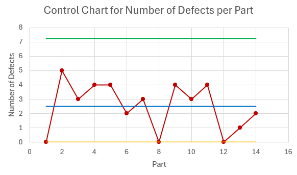
- Calculate the centerline, the upper control limit, and the lower control limit for the [latex]c[/latex]-chart to monitor the number of defects per part at [latex]99.7\%[/latex] confidence.
- Construct the [latex]c[/latex]-chart. Is the process in-control? Explain.
Solution
- First, calculate the mean of the number of defects per part.
[latex]\begin{eqnarray*}\\\overline{c}&=&\frac{0+5+3+4+4+2+3+0+4+3+4+0+1+2}{14}\\&=&2.5\text{ defects per part}\end{eqnarray*}[/latex]
At [latex]99.7\%[/latex] confidence [latex]z=3[/latex].
[latex]\begin{eqnarray*}\text{Centerline}&=&\overline{c}\\&=&2.5\text{ defects per part}\\\\\text{Upper Control Limit}&=&\overline{c}+z\times\sqrt{\overline{c}}\\&=&2.5+3\times\sqrt{2.5}\\&=&7.24\text{ defects per part}\\\\\text{Lower Control Limit}&=&\overline{c}-z\times\sqrt{\overline{c}}\\&=&2.5-3\times\sqrt{2.5}\\&=&-2.24\rightarrow 0\text{ defects per part}\\\end{eqnarray*}[/latex]
- The [latex]c[/latex]-chart is
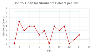
Based on the control chart, the number of defects per part appears to be in-control.
NOTES
- Because this chart is for [latex]99.7\%[/latex] confidence, the value of [latex]z[/latex] in the formulas for the upper and lower control limits is [latex]3[/latex]. This sets the upper and lower control limits at [latex]3[/latex] standard deviations above and below the centerline, respectively.
- When the formula for the lower control limit in a [latex]c[/latex]-chart produces a negative number, the lower control limit is set to [latex]0[/latex]. Because the [latex]c[/latex]-chart monitors the number of defects, it does not make sense to have a negative lower control limit, and so the convention in such cases is to make the lower control limit equal to [latex]0[/latex].
- Use Excel to find the average of the number of defects column.
- On the [latex]c[/latex]-chart, we plot the number of defects per item.
TRY IT
A company produces five products per hour. The company wants to track the number of defects in each hour's batch of product. Over the course of a 10-hour production cycle, the number of defects each hour was recorded in the table below. Calculate the centerline, the upper control limit, and the lower control limit for the control chart to monitor the number of defects per hour at [latex]99.7\%[/latex] confidence.
| Hour | Number of Defects |
|---|---|
| 1 | 2 |
| 2 | 1 |
| 3 | 3 |
| 4 | 0 |
| 5 | 3 |
| 6 | 2 |
| 7 | 1 |
| 8 | 2 |
| 9 | 3 |
| 10 | 2 |
Click to see Solution
[latex]\begin{eqnarray*}\\\overline{c}&=&\frac{2+1+3+0+3+3+2+1+2+3+2}{10}\\&=&1.9\text{ defects per hour}\end{eqnarray*}[/latex]
[latex]\begin{eqnarray*}\\\text{Centerline}&=&\overline{c}\\&=&1.9\text{ defects per hour}\\\\\text{Upper Control Limit}&=&\overline{c}+z\times\sqrt{\overline{c}}\\&=&1.9+3\times\sqrt{1.9}\\&=&6.035\text{ defects per hour}\\\\\text{Lower Control Limit}&=&\overline{c}-z\times\sqrt{\overline{c}}\\&=&1.9-3\times\sqrt{1.9}\\&=&-2.235\rightarrow 0\text{ defects per hour}\\\end{eqnarray*}[/latex]
Exercises
- A company produces marble countertops. A defect in the countertop requires the entire countertop to be reconstructed. In a sample of [latex]80[/latex] countertops, [latex]3[/latex] were defective. Calculate the centerline, upper control limit, and lower control limit for the control chart to monitor the percentage of defective countertops at [latex]95\%[/latex] confidence.
Click to see Answer
[latex]\text{Centerline}=3.75\%[/latex], [latex]\text{Upper Control Limit}=7.998\%[/latex], [latex]\text{Lower Control Limit}=0\%[/latex]
- A retail store monitors the number of customer returns per day. Under normal conditions, the store expects [latex]12[/latex] customer returns per day.
- Calculate the centerline, upper control limit, and lower control limit for the control chart to monitor the number of customer returns per day at [latex]99.7\%[/latex] confidence.
- Over the past two weeks, the store recorded the following number of customer returns per day: [latex]4[/latex], [latex]15[/latex], [latex]14[/latex], [latex]8[/latex], [latex]20[/latex], [latex]24[/latex], [latex]5[/latex], [latex]13[/latex], [latex]11[/latex], [latex]25[/latex], [latex]6[/latex], [latex]7[/latex], [latex]16[/latex], [latex]11[/latex]. Construct the control chart to monitor the number of customer returns per day.
- Is the process in-control? Ex lain.
Click to see Answer
- [latex]\text{Centerline}=12\text{ returns per day}[/latex], [latex]\text{Upper Control Limit}=22.39\text{ returns per day}[/latex], [latex]\text{Lower Control Limit}=1.61\text{ returns per day}[/latex]
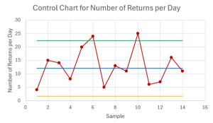
- The process is out-of-control because there are points above the upper control limit.
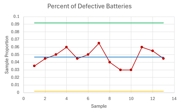
- A company manufactures batteries. The quality control department monitors the percentage of defective batteries produced each day. A quality control inspector takes a sample of [latex]200[/latex] batteries over a 13-day period and records the number of defective batteries in each sample. The data is recorded in the table below.
Day Number of Defective Batteries 1 7 2 9 3 10 4 12 5 9 6 10 7 13 8 8 9 6 10 6 11 12 12 11 13 9 - Calculate the centerline, upper control limit, and lower control limit to monitor the percent of defective batteries made each day at [latex]99.7\%[/latex] confidence.
- Construct the control chart to monitor the percentage of defective batteries.
- Is the process in-control? Exp ain.
Click to see Answer
- [latex]\text{Centerline}=4.69\%[/latex], [latex]\text{Upper Control Limit}=9.18\%[/latex], [latex]\text{Lower Control Limit}=0.21\%[/latex]

- Based on the [latex]p[/latex]-chart, the process appears in-control.
- A retail store receives complaints about the attitude of some of its sales associates. Over a 10-day period, the store records the number of complaints they receive per day. The data is recorded in the table below. Calculate the centerline, upper control limit, and lower control limit for the control chart to monitor the number of complaints per day at [latex]95\%[/latex] confidence.
Day Number of Complaints 1 22 2 23 3 25 4 24 5 28 6 23 7 20 8 27 9 25 10 23 Click to see Answer
[latex]\text{Centerline}=24\text{ complaints per day}[/latex], [latex]\text{Upper Control Limit}=33.798\text{ complaints per day}[/latex], [latex]\text{Lower Control Limit}=14.202\text{ complaints per day}[/latex]
- A computer software manufacturer offers its customers a 24-hour helpline if they have problems or questions about the software. In one 24-hour period, the company received [latex]384[/latex] calls to its helpline. Calculate the centerline, upper control limit, and lower control limit for the control chart to monitor the number of calls per hour to the helpline with [latex]99.7\%[/latex] confidence.
Click to see Answer
[latex]\text{Centerline}=16\text{ calls per hour}[/latex], [latex]\text{Upper Control Limit}=28\text{ calls per hour}[/latex], [latex]\text{Lower Control Limit}=4\text{ calls per hour}[/latex]
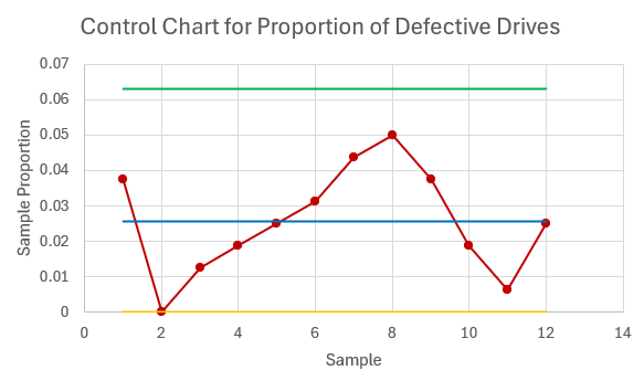
- A manufacturer of flash drives wants to monitor the percentage of defective drives produced. Over a 10-day period, the manufacturer takes a sample of [latex]160[/latex] drives each day and tests each drive. The proportion of defective drives in each sample is recorded in the table below.
Sample Proportion Defective 1 0.0375 2 0 3 0.0125 4 0.01875 5 0.025 6 0.03125 7 0.04375 8 0.05 9 0.0375 10 0.01875 11 0.00625 12 0.025 - Calculate the centerline, upper control limit, and lower control limit to monitor the proportion of defective drives made each day at [latex]99.7\%[/latex] confidence.
- Construct the control chart to monitor the proportion of defective batteries.
- Is the process in-control? Exp ain.
Click to see Answer
- [latex]\text{Centerline}=2.55\%[/latex], [latex]\text{Upper Control Limit}=6.29\%[/latex], [latex]\text{Lower Control Limit}=0\%[/latex]
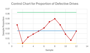
- Based on the [latex]p[/latex]-chart, the process appears out-of-control because there are six consecutive increasing points.