15.2 Control Charts for Variables
LEARNING OBJECTIVES
- Calculate the centerline, upper control limit, and lower control limit for an [latex]\overline{x}[/latex]-chart or an [latex]R[/latex]-chart.
Control charts that are used to monitor processes that are measured on a continuous scale are called control charts for variables. Examples of measurements that might require monitoring include weight, height, or volume. There are two different types of control charts to monitor measurements—control charts for means and control charts for range. Control charts for means, called [latex]\overline{x}[/latex]-charts, monitor the mean or central tendency of the process. For example, if a company produces [latex]300[/latex] gram bags of ground coffee, the [latex]\overline{x}[/latex]-chart monitors the mean weight of the bags of coffee. Control charts for range, called [latex]R[/latex]-charts, monitor the variability of the process. For example, if a company produces [latex]300[/latex] gram bags of ground coffee, the [latex]R[/latex]-chart monitors the range between the heaviest weight and the lightest weight of the bags of coffee. Generally, [latex]\overline{x}[/latex]-charts and [latex]R[/latex]-charts are used together in order to monitor both the average and variability of the process simultaneously.
[latex]\overline{x}[/latex]-Charts
An [latex]\overline{x}[/latex]-chart monitors the average or central tendency of a process. To construct an [latex]\overline{x}[/latex]-chart, a collection of samples, all of the same size [latex]n[/latex], are taken from the process; the mean of each sample is calculated, and the sample means are plotted on the control chart. Because an [latex]\overline{x}[/latex]-chart is based on samples taken from a population, [latex]\overline{x}[/latex]-charts are based on the sampling distribution of the sample means and the Central Limit Theorem.
Recall that the sampling distribution of the sample means [latex]\overline{x}[/latex] is the distribution of the sample means from all possible samples of size [latex]n[/latex] taken from a population. The Central Limit Theorem states that the distribution of the sample means follows a normal distribution if the population the samples are taken from is normal or if the sample size [latex]n[/latex] is sufficiently large (i.e. [latex]n\geq30[/latex]). As well, the theorem states that
[latex]\displaystyle{\mu_{\overline{x}}=\mu\;\;\;\;\;\;\;\;\;\;\sigma_{\overline{x}}=\frac{\sigma}{\sqrt{n}}}[/latex]
where [latex]\mu_{\overline{x}},[/latex] is the mean of the sample means, [latex]\sigma_{\overline{x}}[/latex] is the standard deviation of the sample means, [latex]\mu[/latex] is the population mean, [latex]\sigma[/latex] is the population standard deviation, and [latex]n[/latex] is the sample size.
Recall that the Empirical Rule for normal distributions states that [latex]95\%[/latex] of the observations fall within two standard deviations of the mean and [latex]99.7\%[/latex] of the observations fall within three standard deviations of the mean. Assuming the conditions of the Central Limit Theorem are met, the distribution of the sample means follows a normal distribution. So the Empirical Rule applies to the distribution of the sample means, and implies that:
- [latex]95\%[/latex] of the sample means [latex]\overline{x}[/latex] fall within two standard deviations [latex]\sigma_{\overline{x}}[/latex] of the mean [latex]\mu_{\overline{x}}[/latex]. In other words, [latex]95\%[/latex] of the sample means fall in between the values of [latex]\mu_{\overline{x}}-2\sigma_{\overline{x}}[/latex] and [latex]\mu_{\overline{x}}+2\sigma_{\overline{x}}[/latex].
- [latex]99.7\%[/latex] of the sample means [latex]\overline{x}[/latex] fall within three standard deviations [latex]\sigma_{\overline{x}}[/latex] of the mean [latex]\mu_{\overline{x}}[/latex]. In other words, [latex]99.7\%[/latex] of the sample means fall in between the values of [latex]\mu_{\overline{x}}-3\sigma_{\overline{x}}[/latex] and [latex]\mu_{\overline{x}}+3\sigma_{\overline{x}}[/latex].
This application of the Empirical Rule to the distribution of the sample means forms the basis for the upper and lower control limits on an [latex]\overline{x}[/latex]-chart. In the context of quality control and an [latex]\overline{x}[/latex]-chart, if the sample mean [latex]\overline{x}[/latex] falls within three standard deviations above or below the mean value, then the process is considered in-control with [latex]99.7\%[/latex] confidence. In other words, if a sample mean falls outside the three standard deviations, then the process is out-of-control with [latex]99.7\%[/latex] confidence. Similarly, if the sample mean [latex]\overline{x}[/latex] falls within two standard deviations above or below the mean value, then the process is considered in-control with [latex]95\%[/latex] confidence.
Process Mean and Process Standard Deviation Known
The process mean is the population mean [latex]\mu[/latex], and the process standard deviation is the population standard deviation [latex]\sigma[/latex]. When both of these values are known, [latex]\mu_{\overline{x}}=\mu[/latex] and [latex]\sigma_{\overline{x}}=\frac{\sigma}{\sqrt{n}}[/latex]. Then the centerline, the upper control limit, and the lower control limit for the [latex]\overline{x}[/latex]-chart are:
[latex]\begin{eqnarray*}\text{Centerline}&=&\mu\\\text{Upper Control Limit}&=&\mu+z\times\frac{\sigma}{\sqrt{n}}\\\text{Lower Control Limit}&=&\mu-z\times\frac{\sigma}{\sqrt{n}}\\\\\mu&=&\text{process mean}\\\sigma&=&\text{process standard deviation}\\n&=&\text{sample size}\\z&=&\text{number of standard deviations}\\&&(2\text{ for }95\%\text{ confidence and }3\text{ for }99.7\%\text{ confidence})\end{eqnarray*}[/latex]
EXAMPLE
A company produces [latex]300[/latex] gram bags of ground coffee. To monitor the average weight of the bags, [latex]36[/latex] bags are selected every hour and weighed. Based on an analysis of old records, the standard deviation of the overall weight of the bags is estimated to be [latex]8[/latex] grams.
- At [latex]99.7\%[/latex] confidence, calculate the centerline, the upper control limit, and the lower control limit for the [latex]\overline{x}[/latex]-chart to monitor the average weight of the bags.
- Suppose the sample means for samples taken over a 10-hour period are [latex]303[/latex], [latex]301[/latex], [latex]302[/latex], [latex]300[/latex], [latex]294[/latex], [latex]297[/latex], [latex]299[/latex], [latex]301[/latex], [latex]298[/latex], [latex]303[/latex]. Construct the [latex]\overline{x}[/latex]-chart. Is the mean of the process in-control? Explain.
Solution
- From the question, we have [latex]\mu=300[/latex], [latex]\sigma=8[/latex] and [latex]n=36[/latex]. At [latex]99.7\%[/latex] confidence, [latex]z=3[/latex].
[latex]\begin{eqnarray*}\\\text{Centerline}&=&\mu\\&=&300\text{ grams}\\\\\text{Upper Control Limit}&=&\mu+z\times\frac{\sigma}{\sqrt{n}}\\&=&300+3\times\frac{8}{\sqrt{36}}\\&=&304\text{ grams}\\\\\text{Lower Control Limit}&=&\mu-z\times\frac{\sigma}{\sqrt{n}}\\&=&300-3\times\frac{8}{\sqrt{36}}\\&=&296\text{ grams}\\\end{eqnarray*}[/latex]
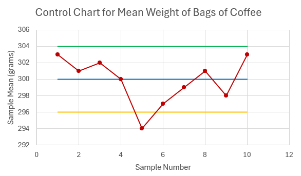
- The [latex]\overline{x}[/latex]-chart is
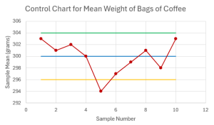
The mean of the fifth sample falls below the lower control limit. This is strong evidence that the mean of the process is out-of-control.
NOTES
- The sample means follow a normal distribution because the sample size [latex]36[/latex] is greater than [latex]30[/latex].
- Because this chart is for [latex]99.7\%[/latex] confidence, the value of [latex]z[/latex] in the formulas for the upper and lower control limits is [latex]3[/latex]. This sets the upper and lower control limits at [latex]3[/latex] standard deviations above and below the centerline, respectively.
- The units for the centerline, upper control limit, and lower control limit are the same units as the data. In this example, the data is measured in grams, so the units of the centerline, upper control limit, and lower control limit are also in grams.
TRY IT
A company produces [latex]30[/latex] cm long metal rods. To monitor the average length of the rods, [latex]40[/latex] rods are selected every hour, and their length is measured. Based on an analysis of old records, the standard deviation of the overall length of the rods is estimated to be [latex]0.5[/latex] cm. At [latex]95\%[/latex] confidence, calculate the centerline, the upper control limit, and the lower control limit for the [latex]\overline{x}[/latex]-chart to monitor the average length of the rods.
Click to see Solution
[latex]\begin{eqnarray*}\\\text{Centerline}&=&\mu\\&=&30\text{ cm}\\\\\text{Upper Control Limit}&=&\mu+z\times\frac{\sigma}{\sqrt{n}}\\&=&30+2\times\frac{0.5}{\sqrt{40}}\\&=&30.16\text{ cm}\\\\\text{Lower Control Limit}&=&\mu-z\times\frac{\sigma}{\sqrt{n}}\\&=&30-2\times\frac{0.5}{\sqrt{40}}\\&=&29.84\text{ cm}\\\end{eqnarray*}[/latex]
Process Mean Unknown and Process Standard Deviation Known
In many situations, the process mean is unknown. In these situations, the process mean [latex]\mu[/latex] is estimated using the mean of the sample means, called the overall sample mean [latex]\overline{\overline{x}}[/latex]. In the process of constructing the [latex]\overline{x}[/latex]-chart, samples are taken and their means calculated. The overall sample mean is just the mean of these sample means.
[latex]\begin{eqnarray*}\overline{\overline{x}}&=&\frac{\overline{x}_1+\overline{x}_2+\cdots+\overline{x}_k}{k}\\\\\overline{x}_j&=&\text{mean of the }j\text{th sample}\\k&=&\text{number of samples}\\\end{eqnarray*}[/latex]
NOTE
The overall sample mean is just the mean of all of the data. Instead of calculating the individual sample means and then calculating the mean of the sample means, the overall sample mean may be found by calculating the average of all of the collected data.
When the process mean is unknown, and the process standard deviation is known, the centerline, the upper control limit, and the lower control limit for the [latex]\overline{x}[/latex]-chart are:
[latex]\begin{eqnarray*}\text{Centerline}&=&\overline{\overline{x}}\\\text{Upper Control Limit}&=&\overline{\overline{x}}+z\times\frac{\sigma}{\sqrt{n}}\\\text{Lower Control Limit}&=&\overline{\overline{x}}-z\times\frac{\sigma}{\sqrt{n}}\\\\\overline{\overline{x}}&=&\text{mean of the sample means}\\\sigma&=&\text{process standard deviation}\\n&=&\text{sample size}\\z&=&\text{number of standard deviations}\\&&(2\text{ for }95\%\text{ confidence and }3\text{ for }99.7\%\text{ confidence})\end{eqnarray*}[/latex]
EXAMPLE
A local beverage company bottles natural spring water. Each day the company takes six samples of [latex]5[/latex] bottles each and measures the volume, in millimeters, of water in the bottles. The data is recorded in the table below. The standard deviation of the overall volume of water in the bottles is estimated to be [latex]10[/latex] ml. Assume the volume of water in each bottle follows a normal distribution.
| Sample | Volume per Bottle | ||||
|---|---|---|---|---|---|
| 1 | 509.31 | 495.97 | 504.4 | 494.89 | 491.6 |
| 2 | 498.51 | 493.81 | 491.52 | 493 | 505.67 |
| 3 | 505.9 | 501.68 | 497.65 | 492.6 | 508.42 |
| 4 | 507.63 | 498.44 | 504.72 | 506.46 | 493.03 |
| 5 | 509.36 | 494.57 | 492.98 | 507.21 | 508.97 |
| 6 | 499.28 | 497.74 | 505.8 | 500.81 | 499.68 |
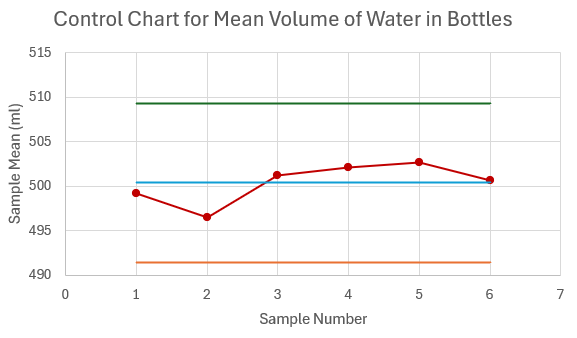
- At [latex]95\%[/latex] confidence, calculate the centerline, the upper control limit, and the lower control limit for the [latex]\overline{x}[/latex]-chart to monitor the mean volume of water in the bottles.
- Construct the [latex]\overline{x}[/latex]-chart. Is the process in-control? Explain.
Solution
- From the questions, we have [latex]\sigma=10[/latex] and [latex]n=5[/latex]. Because the process mean [latex]\mu[/latex] is unknown, we need to calculate [latex]\overline{\overline{x}}[/latex]. For each sample, calculate the sample mean.
Sample Volume per Bottle Sample Mean 1 [latex]509.31[/latex] [latex]495.97[/latex] [latex]504.4[/latex] [latex]494.89[/latex] [latex]491.6[/latex] [latex]499.234[/latex] 2 [latex]498.51[/latex] [latex]493.81[/latex] [latex]491.52[/latex] [latex]493[/latex] [latex]505.67[/latex] [latex]496.502[/latex] 3 [latex]505.9[/latex] [latex]501.68[/latex] [latex]497.65[/latex] [latex]492.6[/latex] [latex]508.42[/latex] [latex]501.25[/latex] 4 [latex]507.63[/latex] [latex]498.44[/latex] [latex]504.72[/latex] [latex]506.46[/latex] [latex]493.03[/latex] [latex]502.056[/latex] 5 [latex]509.36[/latex] [latex]494.57[/latex] [latex]492.98[/latex] [latex]507.21[/latex] [latex]508.97[/latex] [latex]502.618[/latex] 6 [latex]499.28[/latex] [latex]497.74[/latex] [latex]505.8[/latex] [latex]500.81[/latex] [latex]499.68[/latex] [latex]500.662[/latex] Then, the mean of the sample means is
[latex]\begin{eqnarray*}\overline{\overline{x}}&=&\frac{499.234+496.502+501.25+502.056+502.618+500.662}{6}\\&=&500.387 \text{ ml}\end{eqnarray*}[/latex]
At [latex]95\%[/latex] confidence, [latex]z=2[/latex].
[latex]\begin{eqnarray*}\text{Centerline}&=&\overline{\overline{x}}\\&=&500.387\text{ ml}\\\\\text{Upper Control Limit}&=&\overline{\overline{x}}+z\times\frac{\sigma}{\sqrt{n}}\\&=&500.387+2\times\frac{10}{\sqrt{5}}\\&=&509.443\text{ ml}\\\\\text{Lower Control Limit}&=&\overline{\overline{x}}-z\times\frac{\sigma}{\sqrt{n}}\\&=&500.387-2\times\frac{10}{\sqrt{5}}\\&=&491.443\text{ ml}\\\end{eqnarray*}[/latex]
- The [latex]\overline{x}[/latex]-chart is
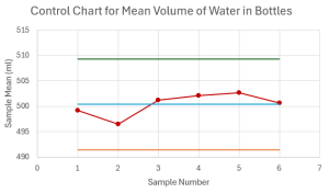
Based on the control chart, the mean of the process appears to be in-control.
NOTES
- The sample means follow a normal distribution because the volume of water in the bottles follows a normal distribution.
- Because this chart is for [latex]95\%[/latex] confidence, the value of [latex]z[/latex] in the formulas for the upper and lower control limits is [latex]2[/latex]. This sets the upper and lower control limits at [latex]2[/latex] standard deviations above and below the centerline, respectively.
- Use Excel to perform the calculations on the raw data, instead of calculating the sample means and overall sample mean by hand.
- The units for the centerline, upper control limit, and lower control limit in an [latex]\overline{x}[/latex]-chart are the same units as the data. In this example, the data is measured in millilitres, so the units of the centerline, upper control limit, and lower control limit are also in millilitres.
- On the [latex]\overline{x}[/latex]-chart, we plot the sample mean for each sample, not the volume for each observation in the sample.
TRY IT
A manufacturer makes round shafts for drill presses. The manufacturer takes a series of samples of [latex]10[/latex] shafts each and measures the diameter, in mm, of each shaft. The sample means for each sample are recorded in the table below. The standard deviation of the overall diameter of the shafts is estimated to be [latex]2.5[/latex] mm. Assume the diameter of the shafts follows a normal distribution. Calculate the centerline, the upper control limit, and the lower control limit for the [latex]\overline{x}[/latex]-chart at [latex]99.7\%[/latex] confidence.
| Sample | Sample Mean |
|---|---|
| 1 | 141.11 |
| 2 | 138.23 |
| 3 | 140.69 |
| 4 | 141.76 |
| 5 | 139.73 |
| 6 | 139.4 |
| 7 | 139.65 |
| 8 | 142.42 |
Click to see Solution
[latex]\begin{eqnarray*}\\\overline{\overline{x}}&=&\frac{141.11+138.23+140.69+141.76+139.73+139.4+139.65+142.43}{8}\\&=&140.37375 \text{ mm}\end{eqnarray*}[/latex]
[latex]\begin{eqnarray*}\\\text{Centerline}&=&\overline{\overline{x}}\\&=&140.37375\text{ mm}\\\\\text{Upper Control Limit}&=&\overline{\overline{x}}+z\times\frac{\sigma}{\sqrt{n}}\\&=&140.37375+3\times\frac{2.5}{\sqrt{10}}\\&=&142.75\text{ mm}\\\\\text{Lower Control Limit}&=&\overline{\overline{x}}-z\times\frac{\sigma}{\sqrt{n}}\\&=&140.37375-3\times\frac{2.5}{\sqrt{10}}\\&=&138\text{ mm}\\\end{eqnarray*}[/latex]
Process Mean and Process Standard Deviation Unknown
In many situations, both the process mean and the process standard deviation are unknown. As above, the process mean [latex]\mu[/latex] is estimated using the overall sample mean [latex]\overline{\overline{x}}[/latex]. Although the average of the sample standard deviations could be used as an estimate of the process standard deviation, in practice, it is more common to use the average range of the samples in the calculation of the control limits for an [latex]\overline{x}[/latex]-chart. Because range is easier to compute, the range can be used as an estimate of the process standard deviation in the [latex]\overline{x}[/latex]-chart calculations with little computational effort.
In the process of constructing the [latex]\overline{x}[/latex]-chart, samples are taken, and their means and ranges are calculated. The average of the sample ranges, [latex]\overline{R}[/latex], is found by averaging the ranges of the samples.
[latex]\begin{eqnarray*}\overline{R}&=&\frac{R_1+R_2+\cdots+R_k}{k}\\\\R_j&=&\text{range of the }j\text{th sample}\\k&=&\text{number of samples}\\\end{eqnarray*}[/latex]
When both the process mean, and the process standard deviation are unknown, the centerline, the upper control limit, and the lower control limit for the [latex]\overline{x}[/latex]-chart are:
[latex]\begin{eqnarray*}\text{Centerline}&=&\overline{\overline{x}}\\\text{Upper Control Limit}&=&\overline{\overline{x}}+A_2\times\overline{R}\\\text{Lower Control Limit}&=&\overline{\overline{x}}-A_2\times\overline{R}\\\\\overline{\overline{x}}&=&\text{mean of the sample means}\\\overline{R}&=&\text{mean of the sample ranges}\\A_2&=&\text{value from Factors for Control Limits Chart}\end{eqnarray*}[/latex]
| Factors for Control Limits Chart | |||
|---|---|---|---|
| Sample Size | [latex]A_2[/latex] | [latex]D_3[/latex] | [latex]D_4[/latex] |
| [latex]2[/latex] | [latex]1.880[/latex] | [latex]0[/latex] | [latex]3.267[/latex] |
| [latex]3[/latex] | [latex]1.023[/latex] | [latex]0[/latex] | [latex]2.575[/latex] |
| [latex]4[/latex] | [latex]0.729[/latex] | [latex]0[/latex] | [latex]2.282[/latex] |
| [latex]5[/latex] | [latex]0.577[/latex] | [latex]0[/latex] | [latex]2.115[/latex] |
| [latex]6[/latex] | [latex]0.483[/latex] | [latex]0[/latex] | [latex]2.004[/latex] |
| [latex]7[/latex] | [latex]0.419[/latex] | [latex]0.076[/latex] | [latex]1.924[/latex] |
| [latex]8[/latex] | [latex]0.373[/latex] | [latex]0.136[/latex] | [latex]1.864[/latex] |
| [latex]9[/latex] | [latex]0.337[/latex] | [latex]0.184[/latex] | [latex]1.816[/latex] |
| [latex]10[/latex] | [latex]0.308[/latex] | [latex]0.223[/latex] | [latex]1.777[/latex] |
| [latex]11[/latex] | [latex]0.285[/latex] | [latex]0.256[/latex] | [latex]1.744[/latex] |
| [latex]12[/latex] | [latex]0.266[/latex] | [latex]0.284[/latex] | [latex]1.716[/latex] |
| [latex]13[/latex] | [latex]0.249[/latex] | [latex]0.308[/latex] | [latex]1.692[/latex] |
| [latex]14[/latex] | [latex]0.235[/latex] | [latex]0.329[/latex] | [latex]1.671[/latex] |
| [latex]15[/latex] | [latex]0.223[/latex] | [latex]0.348[/latex] | [latex]1.652[/latex] |
| [latex]16[/latex] | [latex]0.212[/latex] | [latex]0.364[/latex] | [latex]1.636[/latex] |
| [latex]17[/latex] | [latex]0.203[/latex] | [latex]0.379[/latex] | [latex]1.621[/latex] |
| [latex]18[/latex] | [latex]0.194[/latex] | [latex]0.392[/latex] | [latex]1.608[/latex] |
| [latex]19[/latex] | [latex]0.187[/latex] | [latex]0.404[/latex] | [latex]1.596[/latex] |
| [latex]20[/latex] | [latex]0.180[/latex] | [latex]0.414[/latex] | [latex]1.586[/latex] |
| [latex]21[/latex] | [latex]0.173[/latex] | [latex]0.425[/latex] | [latex]1.575[/latex] |
| [latex]22[/latex] | [latex]0.167[/latex] | [latex]0.434[/latex] | [latex]1.566[/latex] |
| [latex]23[/latex] | [latex]0.162[/latex] | [latex]0.443[/latex] | [latex]1.557[/latex] |
| [latex]24[/latex] | [latex]0.157[/latex] | [latex]0.452[/latex] | [latex]1.548[/latex] |
| [latex]25[/latex] | [latex]0.153[/latex] | [latex]0.459[/latex] | [latex]1.541[/latex] |
NOTES
- The value of [latex]A_2[/latex] in the calculation of the upper and lower control limits in an [latex]\overline{x}[/latex]-chart is based on the sample size.
- The Factors for Control Limits chart is based on [latex]99.7\%[/latex] confidence.
- The process standard deviation [latex]\sigma[/latex] can be estimated by dividing the average range [latex]\overline{R}[/latex] by a constant that depends on the sample size [latex]n[/latex]. The value of [latex]A_2[/latex] results from substituting this estimate for [latex]\sigma[/latex] into the formulas for the control limits with [latex]z=3[/latex].
EXAMPLE
A company produces boxes of cereal. Each day, the company takes five samples of [latex]4[/latex] boxes each and weighs the boxes, in grams, as part of the quality control process. The data is recorded in the table below. Assume the weight of the boxes follows a normal distribution. At [latex]99.7\%[/latex] confidence, calculate the centerline, the upper control limit, and the lower control limit for the [latex]\overline{x}[/latex]-chart to monitor the mean weight of the cereal boxes.
| Sample | Weight of Boxes | |||
|---|---|---|---|---|
| 1 | 503.44 | 497.99 | 501.77 | 502.54 |
| 2 | 495.5 | 495.19 | 499.68 | 503.92 |
| 3 | 497.98 | 501.59 | 500.85 | 499.31 |
| 4 | 498.92 | 498.78 | 502.05 | 497.89 |
| 5 | 503.22 | 502.39 | 500.12 | 499.23 |
Solution
From the questions, we have [latex]n=4[/latex]. Because the process mean [latex]\mu[/latex] and the process standard deviation are unknown, we need to calculate [latex]\overline{\overline{x}}[/latex] and [latex]\overline{R}[/latex]. For each sample, calculate the sample mean and the range.
| Sample | Weight of Boxes | Sample Mean | Sample Range | |||
|---|---|---|---|---|---|---|
| 1 | [latex]503.44[/latex] | [latex]497.99[/latex] | [latex]501.77[/latex] | [latex]502.54[/latex] | [latex]501.435[/latex] | [latex]5.45[/latex] |
| 2 | [latex]495.5[/latex] | [latex]495.19[/latex] | [latex]499.68[/latex] | [latex]503.92[/latex] | [latex]498.5725[/latex] | [latex]8.73[/latex] |
| 3 | [latex]497.98[/latex] | [latex]501.59[/latex] | [latex]500.85[/latex] | [latex]499.31[/latex] | [latex]499.9325[/latex] | [latex]3.61[/latex] |
| 4 | [latex]498.92[/latex] | [latex]498.78[/latex] | [latex]502.05[/latex] | [latex]497.89[/latex] | [latex]499.41[/latex] | [latex]4.16[/latex] |
| 5 | [latex]503.22[/latex] | [latex]502.39[/latex] | [latex]500.12[/latex] | [latex]499.23[/latex] | [latex]501.24[/latex] | [latex]3.99[/latex] |
The mean of the sample means is
[latex]\begin{eqnarray*}\overline{\overline{x}}&=&\frac{501.435+498.5725+499.9325+499.41+501.24}{5}\\&=&500.118 \text{ grams}\end{eqnarray*}[/latex]
The mean of the sample ranges is
[latex]\begin{eqnarray*}\overline{R}&=&\frac{5.45+8.73+3.61+4.16+3.99}{5}\\&=&5.188 \text{ grams}\end{eqnarray*}[/latex]
On the Factors for Control Limits chart, the value for [latex]A_2[/latex] for a sample of size [latex]4[/latex] is [latex]A_2=0.729[/latex].
[latex]\begin{eqnarray*}\text{Centerline}&=&\overline{\overline{x}}\\&=&500.118\text{ grams}\\\\\text{Upper Control Limit}&=&\overline{\overline{x}}+A_2\times\overline{R}\\&=&500.118+0.729\times5.188\\&=&503.90\text{ grams}\\\\\text{Lower Control Limit}&=&\overline{\overline{x}}-A_2\times\overline{R}\\&=&500.118-0.729\times5.188\\&=&496.34\text{ grams}\\\end{eqnarray*}[/latex]
NOTES
- The sample means follow a normal distribution because the weight of the boxes follow a normal distribution.
- Use Excel to perform the calculations on the raw data, instead of calculating the sample means, overall sample mean, sample ranges, and mean of the sample ranges by hand.
- The units for the centerline, upper control limit, and lower control limit are the same units as the data. In this example, the data is measured in grams, so the units of the centerline, upper control limit, and lower control limit are also in grams.
TRY IT
Temperature is used to measure the output from a production process. The company takes [latex]15[/latex] temperature readings, in Celsius, ten times a day as part of the quality control process. The sample means and sample ranges for each sample are recorded in the table below. Assume the temperatures follow a normal distribution. At [latex]99.7\%[/latex] confidence, calculate the centerline, the upper control limit, and the lower control limit for the [latex]\overline{x}[/latex]-chart to monitor the mean temperature of the process.
| Sample | Sample Mean | Sample Range |
|---|---|---|
| 1 | 49.6 | 0.8 |
| 2 | 50.3 | 0.9 |
| 3 | 50.1 | 0.7 |
| 4 | 49.9 | 0.6 |
| 5 | 49.9 | 0.6 |
| 6 | 50.5 | 1 |
| 7 | 50.7 | 0.5 |
| 8 | 49.7 | 0.8 |
| 9 | 49.7 | 0.8 |
| 10 | 50.2 | 0.7 |
Click to see Solution
[latex]\begin{eqnarray*}\\\overline{\overline{x}}&=&\frac{49.6+50.3+50.1+49.9+49.9+50.5+50.7+49.7+49.7+50.2}{10}\\&=&50.06^{\circ}\text{C}\end{eqnarray*}[/latex]
[latex]\begin{eqnarray*}\\\overline{R}&=&\frac{0.8+0.9+0.7+0.6+0.6+1+0.5+0.8+0.8+0.7}{10}\\&=&0.74^{\circ}\text{C}\end{eqnarray*}[/latex]
[latex]\begin{eqnarray*}\\\text{Centerline}&=&\overline{\overline{x}}\\&=&50.06^{\circ}\text{C}\\\\\text{Upper Control Limit}&=&\overline{\overline{x}}+A_2\times\overline{R}\\&=&50.06+0.223\times0.74\\&=&50.23^{\circ}\text{C}\\\\\text{Lower Control Limit}&=&\overline{\overline{x}}-A_2\times\overline{R}\\&=&50.06-0.223\times0.74\\&=&49.89^{\circ}\text{C}\\\end{eqnarray*}[/latex]
[latex]R[/latex]-Charts
An [latex]\overline{x}[/latex]-chart monitors the average or central tendency of a process. However, the variability of the process may be out-of-control, even when the average of the process is in-control. For example, suppose a company produces [latex]300[/latex] gram bags of ground coffee. If the average of the filling process is in-control, the average of the bags of coffee is around [latex]300[/latex] grams. But, if the variability is out-of-control, some bags may be radically underfilled and some bags may be radically overfilled, without changing the average of the process. So in addition to monitoring the average of the process with an [latex]\overline{x}[/latex]-chart, a control chart for the ranges, called an [latex]R[/latex]-chart, is used to monitor the variability of the process. To construct an [latex]R[/latex]-chart, a collection of samples, all of the same size [latex]n[/latex], are taken from the process, the range of each sample is calculated, and the sample ranges are plotted on the control chart.
The centerline, the upper control limit, and the lower control limit for the [latex]R[/latex]-chart are:
[latex]\begin{eqnarray*}\text{Centerline}&=&\overline{R}\\\text{Upper Control Limit}&=&D_4\times\overline{R}\\\text{Lower Control Limit}&=&D_3\times\overline{R}\\\\\overline{R}&=&\text{mean of the sample ranges}\\D_3,D_4&=&\text{values from Factors for Control Limits Chart}\end{eqnarray*}[/latex]
NOTES
- The values of [latex]D_3[/latex] and [latex]D_4[/latex] in the calculation of the upper and lower control limits in an [latex]R[/latex]-chart are based on the sample size.
- Because the Factors for Control Limits chart is based on [latex]99.7\%[/latex] confidence, all [latex]R[/latex]-charts are at [latex]99.7\%[/latex] confidence.
EXAMPLE
A company produces boxes of cereal. Each day, the company takes five samples of [latex]4[/latex] boxes each and weighs the boxes, in grams, as part of the quality control process. The data is recorded in the table below. Assume the weight of the boxes follows a normal distribution.
| Sample | Weight of Boxes | |||
|---|---|---|---|---|
| 1 | 503.44 | 497.99 | 501.77 | 502.54 |
| 2 | 495.5 | 495.19 | 499.68 | 503.92 |
| 3 | 497.98 | 501.59 | 500.85 | 499.31 |
| 4 | 498.92 | 498.78 | 502.05 | 497.89 |
| 5 | 503.22 | 502.39 | 500.12 | 499.23 |
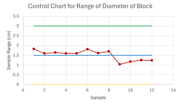
- At [latex]99.7\%[/latex] confidence, calculate the centerline, the upper control limit, and the lower control limit for the [latex]R[/latex]-chart to monitor the variability in the weight of the cereal boxes.
- Construct the [latex]R[/latex]-chart. Is the variability of the process in-control? Explain.
Solution
- From the questions, we have [latex]n=4[/latex]. For each sample, calculate the sample range.
Sample Weight of Boxes Sample Range 1 [latex]503.44[/latex] [latex]497.99[/latex] [latex]501.77[/latex] [latex]502.54[/latex] [latex]5.45[/latex] 2 [latex]495.5[/latex] [latex]495.19[/latex] [latex]499.68[/latex] [latex]503.92[/latex] [latex]8.73[/latex] 3 [latex]497.98[/latex] [latex]501.59[/latex] [latex]500.85[/latex] [latex]499.31[/latex] [latex]3.61[/latex] 4 [latex]498.92[/latex] [latex]498.78[/latex] [latex]502.05[/latex] [latex]497.89[/latex] [latex]4.16[/latex] 5 [latex]503.22[/latex] [latex]502.39[/latex] [latex]500.12[/latex] [latex]499.23[/latex] [latex]3.99[/latex] The mean of the sample ranges is
[latex]\begin{eqnarray*}\overline{R}&=&\frac{5.45+8.73+3.61+4.16+3.99}{5}\\&=&5.188 \text{ grams}\end{eqnarray*}[/latex]
On the Factors for Control Limits chart, the values for [latex]D_3[/latex] and [latex]D_4[/latex] for a sample of size [latex]4[/latex] are [latex]D_3=0[/latex] and [latex]D_4=2.282[/latex].
[latex]\begin{eqnarray*}\text{Centerline}&=&\overline{R}\\&=&5.188\text{ grams}\\\\\text{Upper Control Limit}&=&D_4\times\overline{R}\\&=&2.282\times5.188\\&=&11.839\text{ grams}\\\\\text{Lower Control Limit}&=&D_3\times\overline{R}\\&=&0\times5.188\\&=&0\text{ grams}\\\end{eqnarray*}[/latex]
- The [latex]R[/latex]-chart is
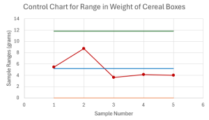
Based on the control chart, the variability of the process appears to be in-control.

NOTES
- Use Excel to perform the calculations on the raw data, instead of calculating the sample ranges and mean of the sample ranges by hand.
- The units for the centerline, upper control limit, and lower control limit for the [latex]R[/latex]-chart are the same units as the data. In this example, the data is measured in grams, so the units of the centerline, upper control limit, and lower control limit are also in grams.
- On the [latex]R[/latex]-chart, we plot the sample ranges for each sample.
TRY IT
Temperature is used to measure the output from a production process. The company takes [latex]15[/latex] temperature readings, in Celsius, ten times a day as part of the quality control process. The sample ranges for each sample are recorded in the table below. Assume the temperatures follow a normal distribution. At [latex]99.7\%[/latex] confidence, calculate the centerline, the upper control limit, and the lower control limit for the [latex]R[/latex]-chart to monitor the variability in the temperature of the process.
| Sample | Sample Range |
|---|---|
| 1 | 0.8 |
| 2 | 0.9 |
| 3 | 0.7 |
| 4 | 0.6 |
| 5 | 0.6 |
| 6 | 1 |
| 7 | 0.5 |
| 8 | 0.8 |
| 9 | 0.8 |
| 10 | 0.7 |
Click to see Solution
[latex]\begin{eqnarray*}\\\overline{R}&=&\frac{0.8+0.9+0.7+0.6+0.6+1+0.5+0.8+0.8+0.7}{10}\\&=&0.74^{\circ}\text{C}\end{eqnarray*}[/latex]
[latex]\begin{eqnarray*}\\\text{Centerline}&=&\overline{R}\\&=&0.74^{\circ}\text{C}\\\\\text{Upper Control Limit}&=&D_R\times\overline{R}\\&=&1.652\times0.74\\&=&1.22248^{\circ}\text{C}\\\\\text{Lower Control Limit}&=&D_3\times\overline{R}\\&=&0.348\times0.74\\&=&0.25752^{\circ}\text{C}\\\end{eqnarray*}[/latex]
Exercises
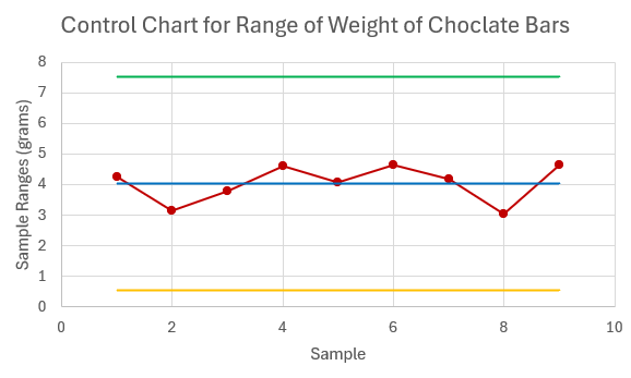
- A company produces chocolate bars. The company wants to monitor the weight, in grams, of the bars. Each day, the company takes nine samples of [latex]8[/latex] chocolate bars and weighs the bars in the sample. The sample means and sample ranges for one day's samples are recorded in the table below. Assume the weights of the bars follow a normal distribution.
Sample Sample Mean Sample Range 1 111.14 4.24 2 112.94 3.15 3 112.42 3.79 4 110.62 4.61 5 112.59 4.08 6 110.04 4.64 7 112.98 4.19 8 113.9 3.05 9 110.3 4.63 - Calculate the centerline, upper control limit, and lower control limit for the control chart to monitor the average weight of the chocolate bars with [latex]99.7\%[/latex] confidence.
- Calculate the centerline, upper control limit, and lower control limit for the control chart to monitor the variability in the weight of the chocolate bars with [latex]99.7\%[/latex] confidence.
- Construct the [latex]\overline{x}[/latex]-chart and [latex]R[/latex]-chart.
- Is the weight of the chocolate bars in-control? Explain.
Click to see Answer
- [latex]\text{Centerline}=111.88\text{ grams}[/latex], [latex]\text{Upper Control Limit}=113.89\text{ grams}[/latex], [latex]\text{Lower Control Limit}=110.37\text{ grams}[/latex]
- [latex]\text{Centerline}=4.04\text{ grams}[/latex], [latex]\text{Upper Control Limit}=7.53\text{ grams}[/latex], [latex]\text{Lower Control Limit}=0.55\text{ grams}[/latex]
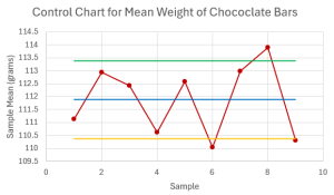

- The average weight of the chocolate bars is out-of-control because there are sample means outside of the control limits on the [latex]\overline{x}[/latex]-chart. The variability of weight appears to be in-control on the [latex]R[/latex]-chart.
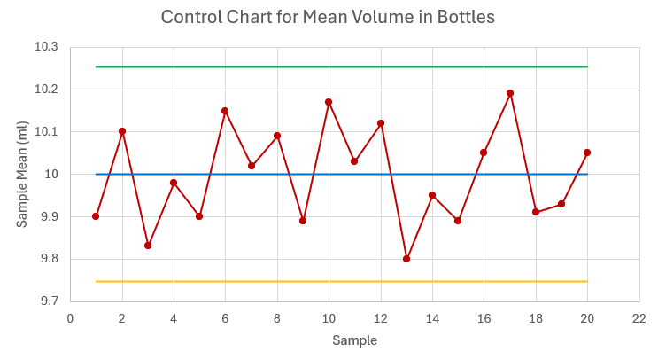
- A cosmetics company produces nail polish. The production process is set up to fill each bottle with [latex]10[/latex] ml of nail polish. The standard deviation of the volume in the bottles is known to be [latex]0.75[/latex] ml. The quality control department periodically selects samples of [latex]35[/latex] bottles and measures the contents.
- Calculate the centerline, upper control limit, and lower control limit for the control chart to monitor the average volume of nail polish in the bottles at [latex]95\%[/latex] confidence.
- Explain what the control limits mean in the context of this question.
- The company takes twenty samples of [latex]35[/latex] bottles. The sample means from the samples are [latex]9.9[/latex], [latex]10.1[/latex], [latex]9.83[/latex], [latex]9.98[/latex], [latex]9.9[/latex], [latex]10.15[/latex], [latex]10.02[/latex], [latex]10.09[/latex], [latex]9.89[/latex], [latex]10.17[/latex], [latex]10.03[/latex], [latex]10.12[/latex], [latex]9.8[/latex], [latex]9.95[/latex], [latex]9.89[/latex], [latex]10.05[/latex], [latex]10.19[/latex], [latex]9.91[/latex], [latex]9.93[/latex], [latex]10.05[/latex]. Construct the [latex]\overline{x}[/latex]-chart.
- Is the process in-control? Explain.
Click to see Answer
- [latex]\text{Centerline}=10\text{ ml}[/latex], [latex]\text{Upper Control Limit}=10.25\text{ ml}[/latex], [latex]\text{Lower Control Limit}=9.75\text{ ml}[/latex]
- [latex]95\%[/latex] of the sample means will fall between [latex]9.75[/latex] ml and [latex]10.25[/latex] ml.
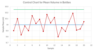
- The process is out-of-control because there are fifteen consecutive points alternating in direction.
- A company manufactures household paint. During a 24-hour production cycle, the company took a sample of [latex]12[/latex] paint cans every hour, and found the overall sample mean of volume in the cans was [latex]3.9[/latex] litres and the mean of the sample ranges was [latex]0.57[/latex] litres.
- Calculate the centerline, upper control limit, and lower control limit for the control chart to monitor the mean volume of paint in the cans at [latex]99.7\%[/latex] confidence.
- Calculate the centerline, upper control limit, and lower control limit for the control chart to monitor the variability of the volume of pain in the cans at [latex]99.7\%[/latex] confidence.
Click to see Answer
- [latex]\text{Centerline}=3.9\text{ liters}[/latex], [latex]\text{Upper Control Limit}=40.5\text{ liters}[/latex], [latex]\text{Lower Control Limit}=3.75\text{ liters}[/latex]
- [latex]\text{Centerline}=0.57\text{ liters}[/latex], [latex]\text{Upper Control Limit}=0.98\text{ liters}[/latex], [latex]\text{Lower Control Limit}=0.16\text{ liters}[/latex]
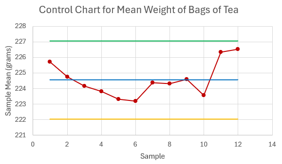
- A tea manufacturer produces bags of loose-leaf tea that it sells to restaurants and coffee shops. As part of the quality control process, the manufacturer takes samples of the bags and measures the weight, in grams, of tea in the bags. The weights from the samples are recorded in the table below. From prior experience, the manufacturer knows that the standard deviation of the weight in the bags is [latex]2.8[/latex] grams.
Sample Weight of Bags of Tea 1 220.92 228.74 224.47 226.74 227.73 2 226.66 227.74 221.94 226.64 220.8 3 224.99 224.18 221.77 226.02 223.85 4 223.17 222.65 221.32 225.63 226.24 5 225.41 222.22 221.42 223.55 223.92 6 222.79 224.98 223.11 221.35 223.78 7 220.65 225.09 224.19 225.76 226.13 8 221.05 223.49 225.85 229.85 221.28 9 227.05 228.59 223.95 220.01 223.32 10 223.35 221.34 223.58 227.31 222.27 11 225.28 227.86 221.88 229.99 226.63 12 225.84 226.31 222.77 228.61 229.17 - Calculate the centerline, upper control limit, and lower control limit for the [latex]\overline{x}[/latex]-chart to monitor the weight of tea in the bags at [latex]95\%[/latex] confidence.
- Construct the [latex]\overline{x}[/latex]-chart.
- Is the weight of the bags of tea in-control? Explain.
Click to see Answer
- [latex]\text{Centerline}=224.55\text{ grams}[/latex], [latex]\text{Upper Control Limit}=227.06\text{ grams}[/latex], [latex]\text{Lower Control Limit}=222.05\text{ grams}[/latex]
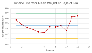
- The weight of the bags of tea is out-of-control because there is a trend of six decreasing points on the control chart.
- A company produces bags of pretzels. To ensure the bags have the proper weight, samples of [latex]49[/latex] bags are taken and each bag is weighed. The overall mean of the samples is [latex]225.17[/latex] grams. The standard deviation of the weights of the bags is [latex]25[/latex] grams. At [latex]99.7\%[/latex] confidence, calculate the centerline, upper control limit, and lower control limit for the control chart to monitor the mean weight of the bags.
Click to see Answer
[latex]\text{Centerline}=225.17\text{ grams}[/latex], [latex]\text{Upper Control Limit}=235.88\text{ grams}[/latex], [latex]\text{Lower Control Limit}=214.46\text{ grams}[/latex]
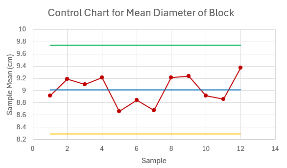
- A company produces cylindrical blocks for a children's toy. The company needs to monitor the diameter, in centimetres, of the block to ensure the block fits into the toy. The company takes a series of samples and measures the diameter of blocks in each sample. The data is recorded in the table below. Assume the diameter of the blocks follows a normal distribution.
Sample Diameter of Blocks 1 9.1 8.66 9.27 8.12 8.4 9.94 2 9.9 9.08 8.31 9.49 8.93 9.44 3 9.87 8.62 8.76 9.71 8.23 9.4 4 9.48 8.79 9.85 8.26 9.27 9.63 5 8.21 9.76 8.16 8.48 8.26 9.06 6 8.67 9.2 8.32 8.94 8.06 9.87 7 8.18 8.48 8.36 9.73 9.17 8.12 8 9.42 9.38 9.37 8.17 9.87 9.05 9 9.81 8.78 9.18 8.9 9.69 9.06 10 9.52 8.6 9.38 8.6 9.06 8.34 11 8.57 8.3 9.55 8.93 8.53 9.27 12 9.57 9.41 9.98 9.4 8.75 9.12 - Calculate the centerline, upper control limit, and lower control limit for the control chart to monitor the mean diameter of the block with [latex]99.7\%[/latex] confidence.
- Calculate the centerline, upper control limit, and lower control limit for the control chart to monitor the variability in the diameter of the block with [latex]99.7\%[/latex] confidence.
- Construct the [latex]\overline{x}[/latex]-chart and [latex]R[/latex]-chart.
- Is the diameter of the blocks in-control? Explain.
Click to see Answer
- [latex]\text{Centerline}=9.015\text{ cm}[/latex], [latex]\text{Upper Control Limit}=9.743\text{ cm}[/latex], [latex]\text{Lower Control Limit}=8.289\text{ cm}[/latex]
- [latex]\text{Centerline}=1.504\text{ cm}[/latex], [latex]\text{Upper Control Limit}=3.014\text{ cm}[/latex], [latex]\text{Lower Control Limit}=0\text{ cm}[/latex]
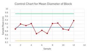
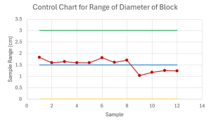
- The average diameter of the blocks appears to be in-control on the [latex]\overline{x}[/latex]-chart. The variability of the diameter appears to be out-of-control on the [latex]R[/latex]-chart because there are eight consecutive points above the centerline.
- Bags of chocolate candy are sampled to ensure proper weight. Ten samples are taken and the weight, in kg, of each bag is recorded in the table below.
Sample Weight of Bags of Candy 1 0.927 0.959 1.074 1.011 0.93 0.952 1.013 1.059 2 0.95 0.947 1.073 1.09 1.025 0.983 1.05 1.09 3 1.095 0.975 0.917 0.941 1.056 0.971 0.947 1.005 4 0.967 1.073 1.086 0.93 1.073 0.967 1.029 0.998 5 0.943 0.988 1.007 1.055 1.031 1.013 0.96 0.91 6 0.932 0.912 1.04 1.084 0.927 1.044 0.938 0.933 7 1.074 0.962 0.92 1.063 0.905 0.911 0.9 0.991 8 0.994 1.049 0.957 0.943 0.962 1.015 1.095 1.028 9 1.072 1.022 1.076 1.02 0.998 0.955 1.019 1.024 10 0.969 0.946 1.019 1.078 1.043 0.931 0.965 0.932 - Calculate the centerline, upper control limit, and lower control limit for the control chart to monitor the mean weight of the bags with [latex]99.7\%[/latex] confidence.
- Calculate the centerline, upper control limit, and lower control limit for the control chart to monitor the variability in the weight of the bags with [latex]99.7\%[/latex] confidence.
Click to see Answer
- [latex]\text{Centerline}=0.9965\text{ kg}[/latex], [latex]\text{Upper Control Limit}=1.0537\text{ kg}[/latex], [latex]\text{Lower Control Limit}=0.9392\text{ kg}[/latex]
- [latex]\text{Centerline}=0.1535\text{ kg}[/latex], [latex]\text{Upper Control Limit}=0.2861\text{ kg}[/latex], [latex]\text{Lower Control Limit}=0.0209\text{ kg}[/latex]