14.5 Regression Models
LEARNING OBJECTIVES
- Construct forecast models using simple linear regression and multiple regression.
A trend pattern is the long-term movement or general direction of the data over a period of time. When a trend is present in a time series, the smoothing models and seasonal indices discussed earlier in this chapter are not able to capture the trend component in the time series, which results in an inaccurate forecast. Instead, we need to use a forecast model that accounts for the trend effect. Although trends do not have to follow a linear model, we will focus on two models that capture the linear trend in a time series.
Linear Trend Projection
Previously, we learned about simple linear regression, which models the linear relationship between an independent variable [latex]x[/latex] and a dependent variable [latex]y[/latex]. The equation for the regression line is
[latex]\begin{eqnarray*}\hat{y}&=&b_0+b_1x\\\\\hat{y}&=&\text{estimated value of }y\\x&=&\text{value of the independent variable}\\b_0&=&y\text{-intercept of the line}\\b_1&=&\text{slope of the line}\end{eqnarray*}[/latex]
We can apply simple linear regression to a time series to model the linear trend in the time series, creating a linear trend projection. A trend line is the simple linear regression equation in which the independent variable [latex]x[/latex] is the time period and [latex]\hat{y}[/latex] is the forecasted value. To emphasize that the independent variable represents time in a trend line model, we will replace the variable [latex]x[/latex] with [latex]t[/latex].
The equation for the trend line is
[latex]\begin{eqnarray*}\hat{y}&=&b_0+b_1t\\\\\hat{y}&=&\text{forecasted value of }y\\t&=&\text{time period}\\b_0&=&y\text{-intercept of the line}\\b_1&=&\text{slope of the line}\end{eqnarray*}[/latex]
The values for the slope [latex]b_1[/latex] and the [latex]y[/latex]-intercept [latex]b_0[/latex] are calculated the same as any simple linear regression equation, using the built-in slope and intercept functions in Excel.
EXAMPLE
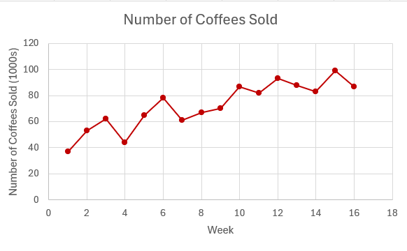
Jane just opened a small coffee shop, located on her town's main street. Jane recorded the number of coffees sold (in [latex]1000[/latex]s) each week for the first 16 weeks since opening the store.
| Week | Number of Coffees Sold ([latex]1000[/latex]s) |
|---|---|
| 1 | 37 |
| 2 | 53 |
| 3 | 62 |
| 4 | 44 |
| 5 | 65 |
| 6 | 78 |
| 7 | 61 |
| 8 | 67 |
| 9 | 70 |
| 10 | 87 |
| 11 | 82 |
| 12 | 93 |
| 13 | 88 |
| 14 | 83 |
| 15 | 99 |
| 16 | 87 |
The time series plot, shown below, shows an upward linear trend. So, the time series has a trend component.
- Create a linear trend projection for this time series.
- Interpret the slope of the linear trend projection.
- Use the linear trend projection to forecast the number of coffees sold for week 17.
- Calculate the [latex]MAD[/latex] for this forecast.
Solution
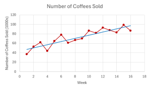
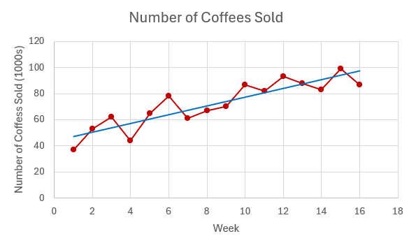
- Using the built-in functions in Excel to calculate the slope and intercept of the trend line, the linear trend projection is:
[latex]\begin{eqnarray*}\\\hat{y}&=&43.85+3.341176\ldots t\\\\\hat{y}&=&\text{forecasted number of coffees in }1000\text{s}\\t&=&\text{time period}\\\end{eqnarray*}[/latex]
- With each additional week, the number of coffees sold increases by [latex]3,341.18[/latex].
- Substitute [latex]t=17[/latex] into the trend line equation:
[latex]\begin{eqnarray*}\\\hat{y}&=&43.85+3.341176\ldots \times 17\\&=&100.65\end{eqnarray*}[/latex]
The forecasted number of coffees sold in week 17 is [latex]100,650[/latex].
-
Week Number of Coffees Sold ([latex]1000[/latex]s) Forecasted Value |Error| 1 [latex]37[/latex] [latex]47.191\ldots[/latex] [latex]10.191\ldots[/latex] 2 [latex]53[/latex] [latex]50.532\ldots[/latex] [latex]2.467\ldots[/latex] 3 [latex]62[/latex] [latex]53.873\ldots[/latex] [latex]8.126\ldots[/latex] 4 [latex]44[/latex] [latex]57.214\ldots[/latex] [latex]13.214\ldots[/latex] 5 [latex]65[/latex] [latex]60.555\ldots[/latex] [latex]4.444\ldots[/latex] 6 [latex]78[/latex] [latex]63.897\ldots[/latex] [latex]14.102\ldots[/latex] 7 [latex]61[/latex] [latex]67.238\ldots[/latex] [latex]6.238\ldots[/latex] 8 [latex]67[/latex] [latex]70.579\ldots[/latex] [latex]3.579\ldots[/latex] 9 [latex]70[/latex] [latex]73.920\ldots[/latex] [latex]3.920\ldots[/latex] 10 [latex]87[/latex] [latex]77.261\ldots[/latex] [latex]9.738\ldots[/latex] 11 [latex]82[/latex] [latex]80.602\ldots[/latex] [latex]1.397\ldots[/latex] 12 [latex]93[/latex] [latex]83.944\ldots[/latex] [latex]9.055\ldots[/latex] 13 [latex]88[/latex] [latex]87.285\ldots[/latex] [latex]0.714\ldots[/latex] 14 [latex]83[/latex] [latex]90.626\ldots[/latex] [latex]7.626\ldots[/latex] 15 [latex]99[/latex] [latex]93.967\ldots[/latex] [latex]5.032\ldots[/latex] 16 [latex]87[/latex] [latex]97.308\ldots[/latex] [latex]10.308\ldots[/latex] Sum [latex]110.158\ldots[/latex] [latex]\begin{eqnarray*}MAD&=&\frac{\sum|\text{forecast error}|}{\text{number of forecast errors}}\\&=&\frac{110.158\ldots}{16}\\&=&6.885\end{eqnarray*}[/latex]
NOTES
- The slope has the same units as the data in the time series. In this case, the data is the number of coffees in [latex]1000[/latex]s. So the slope of [latex]3.341176\ldots[/latex] is in [latex]1000[/latex]s, and is actually [latex]3.341176\ldots\times1000=3,341.17\ldots[/latex].
- The number of coffees sold is given in [latex]1000[/latex]s, so the forecasted values [latex]\hat{y}[/latex] are also in [latex]1000[/latex]s. In the forecasted value for week 17, [latex]\hat{y}=100.65[/latex]. This number is in [latex]1000[/latex]s, so the forecasted number of coffees for week 17 is [latex]100.65\times1000=100,650[/latex].
- In the calculation of the [latex]MAD[/latex], first, find the forecasted value for each week in the time series by substituting the time period into the trend line equation and calculating out [latex]\hat{y}[/latex]. For example, the forecasted value for week 3 is [latex]\hat{y}=43.85+3.341176\ldots \times 3=53.873\ldots[/latex].
NOTES
- Because the trend line is just an application of simple linear regression, we can apply the same measures used in simple linear regression analysis, such as correlation, coefficient of determination, and standard error of the estimate, to assess how well the trend line fits the time series data.
- Unlike the smoothing models, which can only forecast the next time period in the time series, trend lines can be used to forecast further into the future. In the above example, we could use the trend line to create a forecast for week 20 or week 30. However, the further away from the time series data, the less reliable the forecast.
TRY IT
The yearly operating budget (in [latex]\$1,000,000[/latex]s) for a local city is provided in the table below.
| Year | Budget ([latex]\$1,000,000[/latex]s) |
|---|---|
| 1 | 3.14 |
| 2 | 3.27 |
| 3 | 3.33 |
| 4 | 3.45 |
| 5 | 3.68 |
| 6 | 3.76 |
| 7 | 3.98 |
| 8 | 4.05 |
| 9 | 4.12 |
| 10 | 4.47 |
| 11 | 4.65 |
| 12 | 4.78 |
| 13 | 4.82 |
| 14 | 4.85 |
| 15 | 4.93 |
| 16 | 5.02 |
- Create a linear trend projection for this time series.
- Interpret the slope of the linear trend projection.
- Use the linear trend projection to forecast the number of coffees sold for year 20.
Click to see Solution
- [latex]\begin{eqnarray*}\hat{y}&=&2.987\ldots+0.136\ldots t\\\\\hat{y}&=&\text{forecasted budget in }\$1,000,000\text{s}\\t&=&\text{time period}\\\\\end{eqnarray*}[/latex]
- For each additional year, the budget increases by [latex]\$136,058.82[/latex].
- The forecast for year 20 is [latex]\$5,708,426.47[/latex].
Multiple Regression
The linear trend projection discussed above can only handle the trend component of a time series. But many time series include both trend and seasonal components. In such cases, we need to use a forecasting model that incorporates both of these components. One possible model that addresses both trend and seasonal components is a multiple regression model.
Previously, we learned about multiple regression, which models the linear relationship between one dependent variable and several independent variables. The equation for the multiple regression model is:
[latex]\begin{eqnarray*}\hat{y}&=&b_0+b_1x_1+b_2x_2+\cdots+b_kx_k\end{eqnarray*}[/latex]
where [latex]\hat{y}[/latex] is the predicted value of [latex]y[/latex], [latex]x_1,x_2,\ldots,x_k[/latex] are the independent variables, [latex]b_0,b_1,\ldots,b_k[/latex] are the regression coefficients, and [latex]k[/latex] is the number of independent variables.
As with the linear trend projection, [latex]\hat{y}[/latex] in a multiple regression model for a time series is the forecasted value. The number of independent variables in a multiple regression model for a times series equals the number of seasons. For example, a regression model for a time series using quarterly data will have four independent variables because the time series has four seasons. Similarly, a regression model for a time series using monthly data will have twelve independent variables because the time series has twelve seasons. The independent variable [latex]x_1[/latex] is the time period, similar to [latex]t[/latex] in the linear trend projection model above. The remaining independent variables are dummy variables to indicate the season.
NOTE
A dummy variable is a variable that is assigned a value of [latex]1[/latex] if a particular condition is met and a value of [latex]0[/latex] otherwise. In the context of a multiple regression model for a time series, dummy variables are used for the different seasons.
For example, suppose a time series uses quarterly data. The multiple regression model has four independent variables: [latex]x_1, x_2, x_3, x_4[/latex]. The variable [latex]x_1[/latex] is for the time period. The variable [latex]x_2[/latex] is a dummy variable for quarter 2 and equals [latex]1[/latex] when forecasting a quarter 2 value and [latex]0[/latex] otherwise. The variable [latex]x_3[/latex] is a dummy variable for quarter 3 and equals [latex]1[/latex] when forecasting a quarter 3 value and [latex]0[/latex] otherwise. The variable [latex]x_4[/latex] is a dummy variable for quarter 4 and equals [latex]1[/latex] when forecasting a quarter 4 value and [latex]0[/latex] otherwise. When [latex]x_2=x_3=x_4=0[/latex], then the quarter being forecasted is a quarter 1 value.
For a time series with quarterly data, the multiple regression model is
[latex]\begin{eqnarray*}\hat{y}&=&b_0+b_1x_1+b_2x_2+b_3x_3+b_4x_4\\\\\hat{y}&=&\text{forecasted value}\\x_1&=&\text{time period}\\x_2&=&1\text{ if quarter 2 or }0\text{ otherwise}\\x_3&=&1\text{ if quarter 3 or }0\text{ otherwise}\\x_4&=&1\text{ if quarter 4 or }0\text{ otherwise}\\\\\end{eqnarray*}[/latex]
For a time series with monthly data, the multiple regression model is
[latex]\begin{eqnarray*}\hat{y}&=&b_0+b_1x_1+b_2x_2+b_3x_3+\cdots +b_{12}x_{12}\\\\\hat{y}&=&\text{forecasted value}\\x_1&=&\text{time period}\\x_2&=&1\text{ if month 2 or }0\text{ otherwise}\\x_3&=&1\text{ if month 3 or }0\text{ otherwise}\\&\vdots&\\x_{12}&=&1\text{ if month 12 or }0\text{ otherwise}\\\\\end{eqnarray*}[/latex]
In general, for a time series with [latex]k[/latex] seasons, there are [latex]k[/latex] independent variables. The variable [latex]x_1[/latex] is the time period variable, and the variables [latex]x_2,x_3,\ldots,x_k[/latex] are dummy variables.
NOTE
The independent variable that corresponds to the time period is not a dummy variable. The choice of which independent variable corresponds to the time period is arbitrary. In a multiple regression model, the number of independent variables equals the number of seasons. Any of those independent variables can be selected as the time period variable and then the remaining independent variables become dummy variables. The coefficients in the model will be different, but the forecast will be the same regardless of which independent variable is used for the time period. For convenience and consistency, we will designate [latex]x_1[/latex] as the time period variable.
EXAMPLE
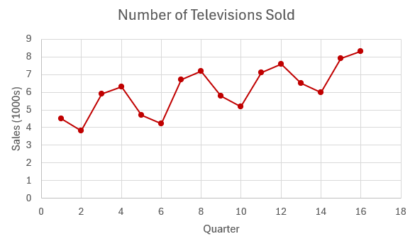
A company makes television sets. The number of sets sold (in [latex]1000[/latex]s) each quarter for the past four years is recorded in the table below.
| Year | Quarter | Sales ([latex]1000[/latex]s) |
|---|---|---|
| 1 | 1 | 4.5 |
| 2 | 3.8 | |
| 3 | 5.9 | |
| 4 | 6.3 | |
| 2 | 5 | 4.7 |
| 6 | 4.2 | |
| 7 | 6.7 | |
| 8 | 7.2 | |
| 3 | 9 | 5.8 |
| 10 | 5.2 | |
| 11 | 7.1 | |
| 12 | 7.6 | |
| 4 | 13 | 6.5 |
| 14 | 6 | |
| 15 | 7.9 | |
| 16 | 8.3 |
The time series plot, shown below, indicates that there are drops in sales in the second quarter of each year and that there are peaks in sales in the third and fourth quarters of each year. The time series plot also shows an upward linear trend. So, the time series has both seasonal and trend components.
- Create a multiple regression model for this time series.
- Use the multiple regression model to forecast the number of televisions sold for each quarter for year 5.
- Calculate the [latex]MAPE[/latex] for this forecast.
Solution
- The time series has four seasons/quarters, so the multiple regression model will have four independent variables: [latex]x_1[/latex] for the time period and dummy variables [latex]x_2,x_3,x_4[/latex] for quarters 2, 3 and 4. To use Excel's regression analysis, we need to set up a table, shown below, containing the values of the independent variables for the data. The values for the time period variable [latex]x_1[/latex] are the time period values. We need to add three additional columns for the dummy variables [latex]x_2,x_3,x_4[/latex]. The values in these additional columns are [latex]1[/latex] for the corresponding quarter or [latex]0[/latex] otherwise. For example, in the Quarter 2 column, there is a [latex]1[/latex] in each row that corresponds to a Quarter 2 (quarters 2, 6, 10, and 14) in the data and a [latex]0[/latex] everywhere else. In the Quarter 3 column, there is a [latex]1[/latex] in each row that corresponds to a Quarter 3 (quarters 3, 7, 11, and 15) in the data and a [latex]0[/latex] everywhere else. In the Quarter 4 column, there is a [latex]1[/latex] in each row that corresponds to a Quarter 4 (quarters 4, 8, 12, and 16) in the data and a [latex]0[/latex] everywhere else.
Time Period Quarter 2 Quarter 3 Quarter 4 Sales ([latex]1000[/latex]s) [latex]1[/latex] [latex]0[/latex] [latex]0[/latex] [latex]0[/latex] [latex]4.5[/latex] [latex]2[/latex] [latex]1[/latex] [latex]0[/latex] [latex]0[/latex] [latex]3.8[/latex] [latex]3[/latex] [latex]0[/latex] [latex]1[/latex] [latex]0[/latex] [latex]5.9[/latex] [latex]4[/latex] [latex]0[/latex] [latex]0[/latex] [latex]1[/latex] [latex]6.3[/latex] [latex]5[/latex] [latex]0[/latex] [latex]0[/latex] [latex]0[/latex] [latex]4.7[/latex] [latex]6[/latex] [latex]1[/latex] [latex]0[/latex] [latex]0[/latex] [latex]4.2[/latex] [latex]7[/latex] [latex]0[/latex] [latex]1[/latex] [latex]0[/latex] [latex]6.7[/latex] [latex]8[/latex] [latex]0[/latex] [latex]0[/latex] [latex]1[/latex] [latex]7.2[/latex] [latex]9[/latex] [latex]0[/latex] [latex]0[/latex] [latex]0[/latex] [latex]5.8[/latex] [latex]10[/latex] [latex]1[/latex] [latex]0[/latex] [latex]0[/latex] [latex]5.2[/latex] [latex]11[/latex] [latex]0[/latex] [latex]1[/latex] [latex]0[/latex] [latex]7.1[/latex] [latex]12[/latex] [latex]0[/latex] [latex]0[/latex] [latex]1[/latex] [latex]7.6[/latex] [latex]13[/latex] [latex]0[/latex] [latex]0[/latex] [latex]0[/latex] [latex]6.5[/latex] [latex]14[/latex] [latex]1[/latex] [latex]0[/latex] [latex]0[/latex] [latex]6[/latex] [latex]15[/latex] [latex]0[/latex] [latex]1[/latex] [latex]0[/latex] [latex]7.9[/latex] [latex]16[/latex] [latex]0[/latex] [latex]0[/latex] [latex]1[/latex] [latex]8.3[/latex] Using this table, apply Excel's regression analysis to find the multiple regression model:
[latex]\begin{eqnarray*}\hat{y}&=&4.171875+0.17875x_1-0.746875x_2+1.18125x_3+1.459375x_4\\\\\hat{y}&=&\text{forecasted sales in }1000\text{s}\\x_1&=&\text{time period}\\x_2&=&1\text{ if quarter 2 or }0\text{ otherwise}\\x_3&=&1\text{ if quarter 3 or }0\text{ otherwise}\\x_4&=&1\text{ if quarter 4 or }0\text{ otherwise}\\\\\end{eqnarray*}[/latex]
- Forecast for quarter 1 of year 5 (time period 17):
[latex]\begin{eqnarray*}\\\hat{y}&=&4.171875+0.17875\times17-0.746875\times0+1.18125\times0+1.459375\times0\\&=&7.09375\end{eqnarray*}[/latex]
The forecasted sales for quarter 1 of year 5 is [latex]7,093.75[/latex].
Forecast for quarter 2 of year 5 (time period 18):
[latex]\begin{eqnarray*}\hat{y}&=&4.171875+0.17875\times18-0.746875\times1+1.18125\times0+1.459375\times0\\&=&6.51875\end{eqnarray*}[/latex]
The forecasted sales for quarter 2 of year 5 is [latex]6,518.75[/latex].
Forecast for quarter 3 of year 5 (time period 19):
[latex]\begin{eqnarray*}\hat{y}&=&4.171875+0.17875\times19-0.746875\times0+1.18125\times1+1.459375\times0\\&=&8.618.75\end{eqnarray*}[/latex]
The forecasted sales for quarter 3 of year 5 is [latex]8,618.75[/latex].
Forecast for quarter 4 of year 5 (time period 20):
[latex]\begin{eqnarray*}\hat{y}&=&4.171875+0.17875\times20-0.746875\times0+1.18125\times0+1.459375\times1\\&=&9,068.75\end{eqnarray*}[/latex]
The forecasted sales for quarter 4 of year 5 is [latex]9,068.75[/latex].
-
Quarter Sales ([latex]1000[/latex]s) Forecasted Value |Percent Error| [latex]1[/latex] [latex]4.5[/latex] [latex]4.34375[/latex] [latex]0.0347\ldots[/latex] [latex]2[/latex] [latex]3.8[/latex] [latex]3.76875[/latex] [latex]0.0082\ldots[/latex] [latex]3[/latex] [latex]5.9[/latex] [latex]5.86875[/latex] [latex]0.0052\ldots[/latex] [latex]4[/latex] [latex]6.3[/latex] [latex]6.31875[/latex] [latex]0.0029\ldots[/latex] [latex]5[/latex] [latex]4.7[/latex] [latex]5.03125[/latex] [latex]0.0704\ldots[/latex] [latex]6[/latex] [latex]4.2[/latex] [latex]4.45625[/latex] [latex]0.0610\ldots[/latex] [latex]7[/latex] [latex]6.7[/latex] [latex]6.55625[/latex] [latex]0.0214\ldots[/latex] [latex]8[/latex] [latex]7.2[/latex] [latex]7.00625[/latex] [latex]0.0269\ldots[/latex] [latex]9[/latex] [latex]5.8[/latex] [latex]5.71875[/latex] [latex]0.0140\ldots[/latex] [latex]10[/latex] [latex]5.2[/latex] [latex]5.14375[/latex] [latex]0.0108\ldots[/latex] [latex]11[/latex] [latex]7.1[/latex] [latex]7.24375[/latex] [latex]0.0202\ldots[/latex] [latex]12[/latex] [latex]7.6[/latex] [latex]7.69375[/latex] [latex]0.0123\ldots[/latex] [latex]13[/latex] [latex]6.5[/latex] [latex]6.40625[/latex] [latex]0.0144\ldots[/latex] [latex]14[/latex] [latex]6[/latex] [latex]5.83125[/latex] [latex]0.0281\ldots[/latex] [latex]15[/latex] [latex]7.9[/latex] [latex]7.93125[/latex] [latex]0.0039\ldots[/latex] [latex]16[/latex] [latex]8.3[/latex] [latex]8.38125[/latex] [latex]0.0097\ldots[/latex] Sum [latex]0.3447\ldots[/latex] [latex]\begin{eqnarray*}MAPE&=&\frac{\sum|\text{percent error}|}{\text{number of forecast errors}}\times100\%\\&=&\frac{0.3447\ldots}{16}\times100\%\\&=&2.15\%\end{eqnarray*}[/latex]
NOTES
- The number of televisions sold is given in [latex]1000[/latex]s, so the forecasted values [latex]\hat{y}[/latex] are also in [latex]1000[/latex]s. In the forecasted value for quarter 1 of year 5, [latex]\hat{y}=7.09375[/latex]. This number is in [latex]1000[/latex]s, so the forecasted number of televisions sold for quarter 1 of year 5 is [latex]7.09375\times1000=7,093.75[/latex].
- In the calculation of the [latex]MAPE[/latex], first find the forecasted value for each quarter in the time series by substituting the time period and corresponding values of the dummy variables into the multiple regression model and calculating out [latex]\hat{y}[/latex]. For example, the forecasted value for quarter 7 is [latex]\hat{y}=4.171875+0.17875\times 7-0.746875\times0+1.18125\times 1+1.459375\times0=6.55625[/latex].
TRY IT
The number of daily calls to emergency services in a small town is given in the table below.
| Week | Day | Number of Calls |
|---|---|---|
| 1 | Sunday | 38 |
| Monday | 25 | |
| Tuesday | 26 | |
| Wednesday | 24 | |
| Thursday | 24 | |
| Friday | 29 | |
| Saturday | 31 | |
| 2 | Sunday | 34 |
| Monday | 25 | |
| Tuesday | 23 | |
| Wednesday | 26 | |
| Thursday | 24 | |
| Friday | 27 | |
| Saturday | 29 | |
| 3 | Sunday | 30 |
| Monday | 24 | |
| Tuesday | 22 | |
| Wednesday | 23 | |
| Thursday | 21 | |
| Friday | 26 | |
| Saturday | 27 |
- Create a multiple regression model for this time series.
- Use the multiple regression model to forecast the number of calls for each day of week 4.
Click to see Solution
- [latex]\begin{eqnarray*}\hat{y}&=&35.959\ldots-0.244\ldots x_1-9.088\ldots x_2-9.843\ldots x_3-8.931\ldots x_4\\&&-10.020\ldots x_5-5.442\ldots x_6-3.530\ldots x_7\\\\\hat{y}&=&\text{forecasted number of calls}\\x_1&=&\text{time period}\\x_2&=&1\text{ if Monday or }0\text{ otherwise}\\x_3&=&1\text{ if Tuesday or }0\text{ otherwise}\\x_4&=&1\text{ if Wednesday or }0\text{ otherwise}\\x_5&=&1\text{ if Thursday or }0\text{ otherwise}\\x_6&=&1\text{ if Friday or }0\text{ otherwise}\\x_7&=&1\text{ if Saturday or }0\text{ otherwise}\\\\\end{eqnarray*}[/latex]
- Forecast for Sunday of week 4 (time period 22):
[latex]\begin{eqnarray*}\\\hat{y}&=&35.959\ldots-0.244\ldots\times 22-9.088\ldots\times 0-9.843\ldots\times 0-8.931\ldots\times 0\\&&-10.020\ldots\times 0-5.442\ldots\times 0-3.530\ldots\times 0\\&=&30.57\end{eqnarray*}[/latex]
Forecast for Monday of week 4 (time period 23):
[latex]\begin{eqnarray*}\hat{y}&=&35.959\ldots-0.244\ldots\times 23-9.088\ldots\times 1-9.843\ldots\times 0-8.931\ldots\times 0\\&&-10.020\ldots\times 0-5.442\ldots\times 0-3.530\ldots\times 0\\&=&21.24\end{eqnarray*}[/latex]
Forecast for Tuesday of week 4 (time period 24):
[latex]\begin{eqnarray*}\hat{y}&=&35.959\ldots-0.244\ldots\times 24-9.088\ldots\times 0-9.843\ldots\times 1-8.931\ldots\times 0\\&&-10.020\ldots\times 0-5.442\ldots\times 0-3.530\ldots\times 0\\&=&20.24\end{eqnarray*}[/latex]
Forecast for Wednesday of week 4 (time period 25):
[latex]\begin{eqnarray*}\hat{y}&=&35.959\ldots-0.244\ldots\times 25-9.088\ldots\times 0-9.843\ldots\times 0-8.931\ldots\times 1\\&&-10.020\ldots\times 0-5.442\ldots\times 0-3.530\ldots\times 0\\&=&20.9\end{eqnarray*}[/latex]
Forecast for Thursday of week 4 (time period 26):
[latex]\begin{eqnarray*}\hat{y}&=&35.959\ldots-0.244\ldots\times 26-9.088\ldots\times 0-9.843\ldots\times 0-8.931\ldots\times 0\\&&-10.020\ldots\times 1-5.442\ldots\times 0-3.530\ldots\times 0\\&=&19.57\end{eqnarray*}[/latex]
Forecast for Friday of week 4 (time period 27):
[latex]\begin{eqnarray*}\hat{y}&=&35.959\ldots-0.244\ldots\times 27-9.088\ldots\times 0-9.843\ldots\times 0-8.931\ldots\times 0\\&&-10.020\ldots\times 0-5.442\ldots\times 1-3.530\ldots\times 0\\&=&23.9\end{eqnarray*}[/latex]
Forecast for Saturday of week 4 (time period 28):
[latex]\begin{eqnarray*}\hat{y}&=&35.959\ldots-0.244\ldots\times 28-9.088\ldots\times 0-9.843\ldots\times 0-8.931\ldots\times 0\\&&-10.020\ldots\times 0-5.442\ldots\times 0-3.530\ldots\times 1\\&=&25.57\end{eqnarray*}[/latex]
Exercises
- A company that makes kitchen appliances has just launched a new convection oven on the market. Using the weekly sales (in thousands of units) for the eight weeks the oven has been on the market, the company created the linear trend model [latex]\hat{y}=19+1.06t[/latex] where [latex]t[/latex] is the time period and [latex]\hat{y}[/latex] is the forecasted sales (in thousands).
- Interpret the slope of the trend line equation.
- Use the trend line to forecast the sales for week 9.
- Use the trend line to forecast the sales for week 12.
Click to see Answer
- For each additional week, the sales increase by [latex]1,060[/latex] units.
- [latex]28,540[/latex]
- [latex]31,720[/latex]
- The number of cars sold each year for a local used car dealership is recorded in the table below.
Year Number of Cars Sold 1 405 2 370 3 289 4 365 5 302 6 315 7 320 8 265 9 278 10 211 - Create a linear trend projection forecast model for this time series.
- Interpret the slope of the trend line equation.
- Calculate the correlation coefficient for the trend line equation.
- Interpret the correlation coefficient found in part c.
- Use the trend line to forecast the sales for year 11.
- Calculate the [latex]MAPE[/latex] for this forecast.
Click to see Answer
- [latex]\hat{y}=399.7333-15.9515t[/latex] where [latex]t[/latex] is the year and [latex]\hat{y}[/latex] is the forecasted number of cars sold.
- For each additional year, the number of cars sold decreases by [latex]15.95[/latex].
- [latex]-0.8495[/latex]
- There is a strong, negative linear relationship between year and sales.
- [latex]224.27[/latex]
- [latex]7.93\%[/latex]
- An industrial cleaning supply company recorded the monthly sales (in [latex]\$1000[/latex]s) of their industrial vacuum cleaner.
Month Sales ([latex]\$1000[/latex]s) 1 12 2 14 3 11 4 15 5 16 6 14 7 17 8 19 9 15 10 17 11 18 12 18 13 21 - Create a linear trend projection forecast model for this time series.
- Interpret the slope of the trend line equation.
- Calculate the correlation coefficient for the trend line equation.
- Interpret the correlation coefficient found in part c.
- Use the trend line to forecast the sales for month 15.
- Calculate the [latex]MSE[/latex] for this forecast.
Click to see Answer
- [latex]\hat{y}=11.653+0.609 t[/latex] where [latex]t[/latex] is the month and [latex]\hat{y}[/latex] is the forecasted sales.
- For each additional month, the sales increase by [latex]\$609.89[/latex].
- [latex]0.8445[/latex]
- There is a strong, positive linear relationship between month and sales.
- [latex]\$20,802.20[/latex]
- [latex]2.094[/latex]
- The number of surgeries performed each quarter at a small hospital is recorded in the table below.
Quarter Number of Surgeries 1 65 2 57 3 52 4 49 5 51 6 50 7 43 8 42 9 44 10 40 - Create a linear trend projection forecast model for this time series.
- Interpret the slope of the trend line equation.
- Use the trend line to forecast the sales for quarter 13.
- Calculate the [latex]MAD[/latex] for this forecast.
Click to see Answer
- [latex]\hat{y}=62.133-2.333t[/latex] where [latex]t[/latex] is the quarter and [latex]\hat{y}[/latex] is the forecasted number of surgeries.
- For each additional quarter, the number of surgeries decreases by [latex]2.333[/latex].
- [latex]31.8[/latex]
- [latex]2.333[/latex]
- Using five years of quarterly revenue data (in [latex]\$1,000,000[/latex]s), a national restaurant chain created the following multiple regression model to forecast the quarterly revenue.
[latex]\begin{eqnarray*}\hat{y}&=&26.71+3.34x_1-4.54x_2-5.89x_3-2.23x_4\\\\\hat{y}&=&\text{quarterly revenue in }\$1,000,000\text{s}\\x_1&=&\text{time period}\\x_2&=&1\text{ if quarter 2 or }0\text{ otherwise}\\x_3&=&1\text{ if quarter 3 or }0\text{ otherwise}\\x_4&=&1\text{ if quarter 4 or }0\text{ otherwise}\\\\\end{eqnarray*}[/latex]
- Use the multiple regression model to forecast the quarterly revenue for quarter 1 of year 6.
- Use the multiple regression model to forecast the quarterly revenue for quarter 3 of year 6.
- Use the multiple regression model to forecast the quarterly revenue for quarter 2 of year 7.
- Use the multiple regression model to forecast the quarterly revenue for quarter 4 of year 7.
Click to see Answer
- [latex]\$96,850,000[/latex]
- [latex]\$97,640,000[/latex]
- [latex]\$109,010,000[/latex]
- [latex]\$118,000,000[/latex]
- A major source of revenue for a country is the sales tax on goods and services. The quarterly revenue, in millions of dollars, generated by the sales tax is recorded in the table below.
Quarter Revenue from Sales Tax ([latex]\$1,000,000[/latex]s) 1 212 2 239 3 299 4 325 5 248 6 277 7 320 8 340 9 270 10 290 11 340 12 389 - Create a multiple regression forecast model for this time series.
- Use the multiple regression model to forecast the revenue for quarter 13.
- Use the multiple regression model to forecast the revenue for quarter 15.
- Use the multiple regression model to forecast the revenue for quarter 20.
- Calculate the [latex]MAD[/latex] for this forecast.
Click to see Answer
- [latex]\begin{eqnarray*}\hat{y}&=&225.476+8.485x_1-8.722x_2+18.091x_3+47.105x_4\\\\\hat{y}&=&\text{forecasted revenue}\\x_1&=&\text{time period}\\x_2&=&1\text{ if quarter 2 or }0\text{ otherwise}\\x_3&=&1\text{ if quarter 3 or }0\text{ otherwise}\\x_4&=&1\text{ if quarter 4 or }0\text{ otherwise}\end{eqnarray*}[/latex]
- [latex]\$336,786,699.11[/latex]
- [latex]\$371,848,134.63[/latex]
- [latex]\$443,289,740.47[/latex]
- [latex]20.06[/latex]
- A customer comment line is staffed from 8:00 am to 4:30 pm, Monday to Friday. The number of calls received every day for the past five weeks are recorded in the table below.
Week Day Number of Calls 1 Monday 35 Tuesday 17 Wednesday 18 Thursday 20 Friday 29 2 Monday 33 Tuesday 16 Wednesday 17 Thursday 16 Friday 28 3 Monday 29 Tuesday 15 Wednesday 13 Thursday 14 Friday 23 4 Monday 27 Tuesday 15 Wednesday 13 Thursday 15 Friday 25 5 Monday 27 Tuesday 14 Wednesday 13 Thursday 12 Friday 22 - Create a multiple regression forecast model for this time series.
- Use the multiple regression model to forecast the number of calls for each day in week 6.
- Calculate the [latex]MAPE[/latex] for this forecast.
Click to see Answer
- [latex]\begin{eqnarray*}\hat{y}&=&33.588-0.308x_1-14.492x_2-14.784x_3-13.8765x_4-3.568x_5\\\\\hat{y}&=&\text{forecasted number of calls}\\x_1&=&\text{time period}\\x_2&=&1\text{ if Tuesday or }0\text{ otherwise}\\x_3&=&1\text{ if Wednesday or }0\text{ otherwise}\\x_4&=&1\text{ if Thursday or }0\text{ otherwise}\\x_5&=&1\text{ if Friday or }0\text{ otherwise}\end{eqnarray*}[/latex]
- [latex]\text{Monday}=25.58[/latex], [latex]\text{Tuesday}=10.78[/latex], [latex]\text{Wednesday}=10.18[/latex], [latex]\text{Thursday}=10.78[/latex], [latex]\text{Friday}=20.78[/latex]
- [latex]5.69\%[/latex]
- Joe runs a lawn and garden supply store. The monthly sales (in [latex]\$100,000[/latex]) for the past two years are recorded in the table below.
Year Month Sales ([latex]\$100,000[/latex]s) 1 January 3 February 4 March 9 April 13 May 25 June 23 July 22 August 20 September 10 October 6 November 4 December 3 2 January 2 February 3 March 2 April 7 May 26 June 30 July 32 August 29 September 10 October 6 November 4 December 3 - Create a multiple regression forecast model for this time series.
- Use the multiple regression model to forecast the monthly sales for March of year 3.
- Use the multiple regression model to forecast the monthly sales for July of year 3.
- Use the multiple regression model to forecast the monthly sales for September of year 3.
- Use the multiple regression model to forecast the monthly sales for December of year 3.
Click to see Answer
- [latex]\begin{eqnarray*}\hat{y}&=&1.917+0.083x_1+0.917x_2+2.833x_3+7.25x_4+22.667x_5+23.583x_6+24x_7\\&&+21.417x_8+6.833x_9+2.75x_{10}+0.667x_{11}-0.417x_{12}\\\\\hat{y}&=&\text{forecasted sales}\\x_1&=&\text{time period}\\x_2&=&1\text{ if February or }0\text{ otherwise}\\x_3&=&1\text{ if March or }0\text{ otherwise}\\x_4&=&1\text{ if April or }0\text{ otherwise}\\x_5&=&1\text{ if May or }0\text{ otherwise}\\x_6&=&1\text{ if June or }0\text{ otherwise}\\x_7&=&1\text{ if July or }0\text{ otherwise}\\x_8&=&1\text{ if August or }0\text{ otherwise}\\x_9&=&1\text{ if September or }0\text{ otherwise}\\x_{10}&=&1\text{ if October or }0\text{ otherwise}\\x_{11}&=&1\text{ if November or }0\text{ otherwise}\\x_{12}&=&1\text{ if December or }0\text{ otherwise}\end{eqnarray*}[/latex]
- [latex]\$700,000[/latex]
- [latex]\$2,850,000[/latex]
- [latex]\$1,150,000[/latex]
- [latex]\$450,000[/latex]
