14.3 Smoothing Models
LEARNING OBJECTIVES
- Construct forecast models using moving averages, weighted moving averages, and exponential smoothing.
Although some time series do not contain trend, seasonal, or cyclical patterns, almost every time series contains some irregular patterns or random variations. In this section, we will discuss three models—moving averages, weighted moving averages, and exponential smoothing—to reduce or "smooth out" the irregular patterns in the time series. Because the purpose of these models is to "smooth out" the random variations, these models are called smoothing models.
The moving averages, weighted moving averages, and exponential smoothing models are only good at "smoothing" out the random variations present in a time series. When random variation is the only component present in the time series, these models generally create accurate forecasts. But these three models have their limitations. For example, these three models can only make a predication about the next time period in the time series, and so they are not appropriate for more long-term forecasts. Also, these smoothing models are not good at modelling any significant trend, seasonal, or cyclical patterns present in the time series. In cases where trend, seasonality, or cycles are present in the time series, a model that deals with those types of patterns should be used to create an accurate forecast.
The three models discussed in this section are called averaging models. In slightly different ways, each model "averages" data from several previous time periods to create a forecast for the next time period. By using an averaging technique, this type of model smooths out extremes or irregularities in the data.
Moving Averages
The moving average model averages the most recent [latex]k[/latex] values in the time series to forecast the next time period.
[latex]\displaystyle{\text{forecast for each time period}=\text{average of the previous }k\text{ observations}}[/latex]
The "moving" part of this model comes from the fact that as new data becomes available, the oldest observation is replaced with the newest observation, and the average is recalculated. So, the average "moves" or "changes" as each new observation becomes available.
Any number of time periods may be used to calculate a moving average forecast, but the number of time periods used in the forecast must be consistent across the model. That is, we cannot do a [latex]3[/latex]-month moving average for part of the forecast and then switch to a [latex]4[/latex]-month moving average for the rest of the forecast. In general, the forecast becomes smoother when more time periods are included in the average. But too much smoothing many suppress other components of the time series. Through the use of technology, such as Excel, it is easy to experiment with different numbers of time periods in a moving average forecast to find the best forecast.
Suppose we want to create a [latex]2[/latex]-month moving average forecast. The first forecast is for the third month and is the average of the time series values from months one and two. The next forecast is for the fourth month and is the average of the time series values from months two and three. In general, the forecast for each month is the average of the values from the previous two months.
EXAMPLE
A local company produces and sells a certain product. The number of units sold each month for a year is recorded in the table below.
| Month | Actual Number of Units Sold |
|---|---|
| January | 83 |
| February | 102 |
| March | 75 |
| April | 125 |
| May | 100 |
| June | 103 |
| July | 118 |
| August | 101 |
| September | 70 |
| October | 99 |
| November | 120 |
| December | 97 |
- Create a [latex]3[/latex]-month moving average forecast for this time series.
- What is the forecast for January of the next year?
- Calculate the [latex]MAD[/latex] for the [latex]3[/latex]-month moving average forecast.
Solution
-
Month Actual Number of Units Sold [latex]3[/latex]-Month Moving Average Forecast January [latex]83[/latex] February [latex]102[/latex] March [latex]75[/latex] April [latex]125[/latex] [latex]86.666\ldots[/latex] May [latex]100[/latex] [latex]100.666\ldots[/latex] June [latex]103[/latex] [latex]100[/latex] July [latex]118[/latex] [latex]109.333\ldots[/latex] August [latex]101[/latex] [latex]107[/latex] September [latex]70[/latex] [latex]107.333\ldots[/latex] October [latex]99[/latex] [latex]96.333\ldots[/latex] November [latex]120[/latex] [latex]90[/latex] December [latex]97[/latex] [latex]96.333\ldots[/latex] January [latex]105.333\ldots[/latex] 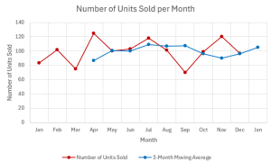
- The forecast for January of the next year is [latex]105.333\ldots[/latex].
-
Month Actual Number of Units Sold [latex]3[/latex]-Month Moving Average Forecast |Forecast Error| January [latex]83[/latex] February [latex]102[/latex] March [latex]75[/latex] April [latex]125[/latex] [latex]86.666\ldots[/latex] [latex]38.333\ldots[/latex] May [latex]100[/latex] [latex]100.666\ldots[/latex] [latex]0.666\ldots[/latex] June [latex]103[/latex] [latex]100[/latex] [latex]3[/latex] July [latex]118[/latex] [latex]109.333\ldots[/latex] [latex]8.666\ldots[/latex] August [latex]101[/latex] [latex]107[/latex] [latex]6[/latex] September [latex]70[/latex] [latex]107.333\ldots[/latex] [latex]37.333\ldots[/latex] October [latex]99[/latex] [latex]96.333\ldots[/latex] [latex]2.666\ldots[/latex] November [latex]120[/latex] [latex]90[/latex] [latex]30[/latex] December [latex]97[/latex] [latex]96.333\ldots[/latex] [latex]0.666\ldots[/latex] January [latex]105.333\ldots[/latex] Sum [latex]127.333\ldots[/latex] [latex]\begin{eqnarray*}MAD&=&\frac{\sum|\text{forecast error}|}{\text{number of forecast errors}}\\&=&\frac{127.333\ldots}{9}\\&=&14.15\end{eqnarray*}[/latex]
NOTES
- To calculate the forecast for April, we average the values from the previous three months:
[latex]\begin{eqnarray*}\\\text{Forecast for April}&=&\frac{83+102+75}{3}=86.666\ldots\end{eqnarray*}[/latex]
To calculate the forecast for May, we average the values from the previous three months:
[latex]\begin{eqnarray*}\text{Forecast for May}&=&\frac{102+75+125}{3}=100.666\ldots\end{eqnarray*}[/latex]
This process continues for each month, averaging the previous three months of observations.
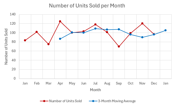
- The graph shows the actual time series data and the [latex]3[/latex]-month moving average forecast. Note how the [latex]3[/latex]-month moving average has smoothed out the monthly variations and indicates the overall trend of the monthly units sold.
- There is no forecast for the first three months. In order to construct a [latex]3[/latex]-month moving average forecast, we need to have three months of prior observations to create the forecast. For January, February, and March, we do not have three months of previous observations, so we cannot create a forecast for those months.
- January of the next year is the last time period that has a forecast because that is the last time period where we have three months of prior observations. We cannot create a forecast for February of the next year because there is no actual value for January of the next year, and so we do not have three months of previous observations.
- In the calculation of the [latex]MAD[/latex], remember that we can only calculate errors when there is an actual value and a forecast value. In this example, there are no errors for January, February, and March because there are no forecasts for those months. Also, there is no error for January of the next year because there is no actual value for that month. Altogether, there are only nine errors, and the [latex]MAD[/latex] is the average of the absolute value of those nine errors.
TRY IT
A local company produces and sells a certain product. The number of units sold each month for a year is recorded in the table below.
| Month | Actual Number of Units Sold |
|---|---|
| January | 83 |
| February | 102 |
| March | 75 |
| April | 125 |
| May | 100 |
| June | 103 |
| July | 118 |
| August | 101 |
| September | 70 |
| October | 99 |
| November | 120 |
| December | 97 |
- Create a [latex]4[/latex]-month moving average forecast for this time series.
- What is the forecast for January of the next year?
- Calculate the [latex]MAD[/latex] for the [latex]4[/latex]-month moving average forecast.
- Which forecast is better: the [latex]3[/latex]-month moving average (from the example above) or the [latex]4[/latex]-month moving average? Why?
Click to see Solution
-
Month Actual Number of Units Sold [latex]4[/latex]-Month Moving Average Forecast |Forecast Error| January [latex]83[/latex] February [latex]102[/latex] March [latex]75[/latex] April [latex]125[/latex] May [latex]100[/latex] [latex]96.25[/latex] [latex]3.75[/latex] June [latex]103[/latex] [latex]100.5[/latex] [latex]2.5[/latex] July [latex]118[/latex] [latex]100.75[/latex] [latex]17.25[/latex] August [latex]101[/latex] [latex]111.75[/latex] [latex]10.5[/latex] September [latex]70[/latex] [latex]105.5[/latex] [latex]35.5[/latex] October [latex]99[/latex] [latex]98[/latex] [latex]1[/latex] November [latex]120[/latex] [latex]97[/latex] [latex]23[/latex] December [latex]97[/latex] [latex]97.5[/latex] [latex]0.5[/latex] January [latex]96.5[/latex] Sum [latex]94[/latex] - The forecast for January of the next year is [latex]96.5[/latex].
- [latex]\displaystyle{MAD=\frac{\sum|\text{forecast error}|}{\text{number of forecast errors}}=\frac{94}{8}=11.75}[/latex]
- The [latex]4[/latex]-month moving average is better because it has the smaller [latex]MAD[/latex].
Weighted Moving Averages
In the moving average model, each observation in the average calculation receives the same weight. But what if we want to apply more emphasis or weight to certain observations and less weight to others? The weighted moving average model applies different pre-set weight to each of the previous values and then calculates the weighted average of the most recent [latex]k[/latex] values in the time series to forecast the next time period.
[latex]\displaystyle{\text{forecast for each time period}=\sum\left[(\text{weight }i)\times(\text{previous value }i)\right]}[/latex]
To calculate the weighted moving average, multiply each observation by its corresponding weight and then add up the results. Typically, more recent observations receive higher weights, giving greater emphasis to more recent values in the time series, and older observations receive lower weights, giving less emphasis to older values in the time series.
For a [latex]k[/latex]-period weighted moving average, the [latex]k[/latex] pre-set weights are applied to the previous [latex]k[/latex] observations. The weights used in a weighted moving average forecast are numbers between [latex]0[/latex] and [latex]1[/latex], and the sum of the weights must equal [latex]1[/latex].
Any number of time periods may be used to calculate a weighted moving average forecast, but the number of time periods used in the forecast must be consistent across the model. The weights must be determined before creating the forecast, and those predetermined weights must be consistent across the entire forecast. Different weights will produce different forecasts. Through the use of technology, such as Excel, it is easy to experiment with different weights and different numbers of time periods in a weighted moving average forecast to find the best forecast.
EXAMPLE
A local company produces and sells a certain product. The number of units sold each month for a year is recorded in the table below.
| Month | Actual Number of Units Sold |
|---|---|
| January | 83 |
| February | 102 |
| March | 75 |
| April | 125 |
| May | 100 |
| June | 103 |
| July | 118 |
| August | 101 |
| September | 70 |
| October | 99 |
| November | 120 |
| December | 97 |
- Create a [latex]3[/latex]-month weighted moving average forecast for this time series. Assign a weight of [latex]0.5[/latex] to the most recent observation, a weight of [latex]0.3[/latex] to the second most recent observation, and a weight of [latex]0.2[/latex] to the third most recent observation.
- What is the forecast for January of the next year?
- Calculate the [latex]MSE[/latex] for the [latex]3[/latex]-month weighted moving average forecast.
Solution
-
Month Actual Number of Units Sold [latex]3[/latex]-Month Weighted Moving Average Forecast January [latex]83[/latex] February [latex]102[/latex] March [latex]75[/latex] April [latex]125[/latex] [latex]84.7[/latex] May [latex]100[/latex] [latex]105.4[/latex] June [latex]103[/latex] [latex]102.5[/latex] July [latex]118[/latex] [latex]106.5[/latex] August [latex]101[/latex] [latex]109.5[/latex] September [latex]70[/latex] [latex]106.5[/latex] October [latex]99[/latex] [latex]88.9[/latex] November [latex]120[/latex] [latex]90.7[/latex] December [latex]97[/latex] [latex]103.7[/latex] January [latex]104.3[/latex] 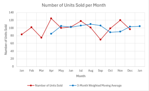
- The forecast for January of the next year is [latex]104.3[/latex].
-
Month Actual Number of Units Sold [latex]3[/latex]-Month Weighted Moving Average Forecast (Forecast Error)2 January [latex]83[/latex] February [latex]102[/latex] March [latex]75[/latex] April [latex]125[/latex] [latex]84.7[/latex] [latex]1624.09[/latex] May [latex]100[/latex] [latex]105.4[/latex] [latex]29.16[/latex] June [latex]103[/latex] [latex]102.5[/latex] [latex]0.25[/latex] July [latex]118[/latex] [latex]106.5[/latex] [latex]132.25[/latex] August [latex]101[/latex] [latex]109.5[/latex] [latex]79.21[/latex] September [latex]70[/latex] [latex]106.5[/latex] [latex]1332.25[/latex] October [latex]99[/latex] [latex]88.9[/latex] [latex]102.01[/latex] November [latex]120[/latex] [latex]90.7[/latex] [latex]858.49[/latex] December [latex]97[/latex] [latex]103.7[/latex] [latex]44.89[/latex] January [latex]104.3[/latex] Sum [latex]4202.6[/latex] [latex]\begin{eqnarray*}MSE&=&\frac{\sum(\text{forecast error})^2}{\text{number of forecast errors}}\\&=&\frac{4202.6}{9}\\&=&466.96\end{eqnarray*}[/latex]
NOTES
- To calculate the forecast for April, we multiply each of the previous three months by their corresponding weights and add up the results:
[latex]\begin{eqnarray*}\\\text{Forecast for April}&=&0.5\times75+0.3\times102+0.2\times83=84.7\end{eqnarray*}[/latex]
To calculate the forecast for May, we multiply each of the previous three months by their corresponding weights and add up the results:
[latex]\begin{eqnarray*}\text{Forecast for May}&=&0.5\times125+0.3\times75+0.2\times102=105.4\end{eqnarray*}[/latex]
This process continues for each month, multiplying each of the previous three months by their corresponding weights and adding up the results.
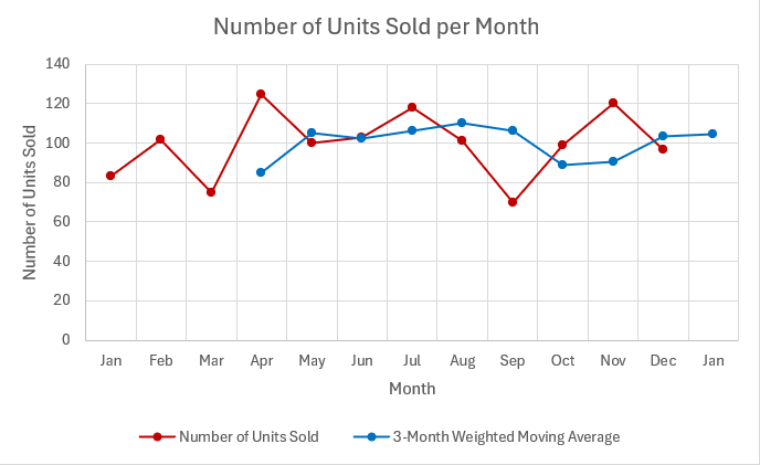
- The graph shows the actual time series data and the [latex]3[/latex]-month weighted moving average forecast. Note how the [latex]3[/latex]-month weighted moving average has smoothed out the monthly variations and indicates the overall trend of the monthly units sold.
- There is no forecast for the first three months. In order to construct a [latex]3[/latex]-month weighted moving average forecast, we need to have three months of prior observations to create the forecast. For January, February, and March, we do not have three months of previous observations, so we cannot create a forecast for those months.
- January of the next year is the last time period that has a forecast because that is the last time period where we have three months of prior observations. We cannot create a forecast for February of the next year because there is no actual value for January of the next year, and so we do not have three months of previous observations.
- In the calculation of the [latex]MSE[/latex], remember that we can only calculate errors when there is an actual value and a forecast value. In this example, there are no errors for January, February, and March because there are no forecasts for those months. Also, there is no error for January of the next year because there is no actual value for that month. Altogether, there are only nine errors, and the [latex]MSE[/latex] is the average of the squares of those nine errors.
TRY IT
A local company produces and sells a certain product. The number of units sold each month for a year is recorded in the table below.
| Month | Actual Number of Units Sold |
|---|---|
| January | 83 |
| February | 102 |
| March | 75 |
| April | 125 |
| May | 100 |
| June | 103 |
| July | 118 |
| August | 101 |
| September | 70 |
| October | 99 |
| November | 120 |
| December | 97 |
- Create a [latex]5[/latex]-month weighted moving average forecast for this time series. Assign a weight of [latex]0.4[/latex] to the most recent observation, a weight of [latex]0.2[/latex] to the second and third most recent observation, and a weight of [latex]0.1[/latex] to the fourth and fifth most recent observation.
- What is the forecast for January of the next year?
- Calculate the [latex]MSE[/latex] for the [latex]5[/latex]-month weighted moving average forecast.
- Which forecast is better: the [latex]3[/latex]-month weighted moving average (from the example above) or the [latex]5[/latex]-month weighted moving average? Why?
Click to see Solution
-
Month Actual Number of Units Sold [latex]5[/latex]-Month Weighted Moving Average Forecast (Forecast Error)2 January [latex]83[/latex] February [latex]102[/latex] March [latex]75[/latex] April [latex]125[/latex] May [latex]100[/latex] June [latex]103[/latex] [latex]98.5[/latex] [latex]20.25[/latex] July [latex]118[/latex] [latex]103.9[/latex] [latex]198.81[/latex] August [latex]101[/latex] [latex]107.8[/latex] [latex]46.24[/latex] September [latex]70[/latex] [latex]107.1[/latex] [latex]1376.41[/latex] October [latex]99[/latex] [latex]92.1[/latex] [latex]47.61[/latex] November [latex]120[/latex] [latex]95.9[/latex] [latex]580.81[/latex] December [latex]97[/latex] [latex]103.7[/latex] [latex]44.89[/latex] January [latex]99.7[/latex] Sum [latex]2315.02[/latex] - The forecast for January of the next year is [latex]99.7[/latex].
- [latex]\displaystyle{MSE=\frac{\sum(\text{forecast error})^2}{\text{number of forecast errors}}=\frac{2315.02}{7}=330.72}[/latex]
- The [latex]5[/latex]-month weighted moving average is better because it has the smaller [latex]MSE[/latex].
Exponential Smoothing
The exponential smoothing model is a special case of a weighted moving average model. In an exponential smoothing model there is only one weight—the weight for the most recent observation. The weight given to the most recent observation, denoted by [latex]\alpha[/latex], is called the smoothing constant. The remaining weight, [latex]1-\alpha[/latex], is applied to the previous forecast.
[latex]\displaystyle{\text{forecast for each time period}=\alpha\times(\text{previous value})+(1-\alpha)\times(\text{previous forecast})}[/latex]
In exponential smoothing, the weighting on the other values decrease exponentially as the observations move further away from the forecasted time period. These other weights are calculated automatically by the formula—all we need to produce an exponential smoothing forecast is the value of smoothing constant [latex]\alpha[/latex].
The smoothing constant [latex]\alpha[/latex] is a pre-set weight and is a number between [latex]0[/latex] and [latex]1[/latex]. A larger value of [latex]\alpha[/latex] places more emphasis on the most recent observation, and a smaller value of [latex]\alpha[/latex] places less emphasis on the most recent observation. The smoothing constant must be determined before creating the forecast, and the value of the smoothing constant must be consistent across the entire forecast. Different values of the smoothing constant will produce different forecasts. Through the use of technology, such as Excel, it is easy to experiment with different values of the smoothing constant in an exponential smoothing forecast to find the best forecast.
NOTE
To create an exponential smoothing forecast, an initial forecast value is needed for the first time period. In some instances, an initial forecast value may be provided. If no initial forecast value is given, use the actual time series value from the first time period as the initial forecast.
EXAMPLE
A local company produces and sells a certain product. The number of units sold each month for a year is recorded in the table below.
| Month | Actual Number of Units Sold |
|---|---|
| January | 83 |
| February | 102 |
| March | 75 |
| April | 125 |
| May | 100 |
| June | 103 |
| July | 118 |
| August | 101 |
| September | 70 |
| October | 99 |
| November | 120 |
| December | 97 |
- Create an exponential smoothing forecast for this time series. Use a smoothing constant of [latex]0.4[/latex] and an initial forecast of [latex]80[/latex].
- What is the forecast for January of the next year?
- Calculate the [latex]MAPE[/latex] for the exponential smoothing forecast.
Solution
-
Month Actual Number of Units Sold Exponential Smoothing Forecast January [latex]83[/latex] [latex]80[/latex] February [latex]102[/latex] [latex]81.2[/latex] March [latex]75[/latex] [latex]89.52[/latex] April [latex]125[/latex] [latex]83.712[/latex] May [latex]100[/latex] [latex]100.227\ldots[/latex] June [latex]103[/latex] [latex]100.136\ldots[/latex] July [latex]118[/latex] [latex]101.281\ldots[/latex] August [latex]101[/latex] [latex]107.969\ldots[/latex] September [latex]70[/latex] [latex]105.181\ldots[/latex] October [latex]99[/latex] [latex]91.108\ldots[/latex] November [latex]120[/latex] [latex]94.265\ldots[/latex] December [latex]97[/latex] [latex]104.559\ldots[/latex] January [latex]101.535\ldots[/latex] 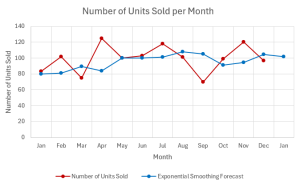
- The forecast for January of the next year is [latex]101.535\ldots[/latex].
-
Month Actual Number of Units Sold Exponential Smoothing Forecast |Percent Error| January [latex]83[/latex] [latex]80[/latex] [latex]0.0361\ldots[/latex] February [latex]102[/latex] [latex]81.2[/latex] [latex]0.2039\ldots[/latex] March [latex]75[/latex] [latex]89.52[/latex] [latex]0.1936[/latex] April [latex]125[/latex] [latex]83.712[/latex] [latex]0.3303\ldots[/latex] May [latex]100[/latex] [latex]100.227\ldots[/latex] [latex]0.0022\ldots[/latex] June [latex]103[/latex] [latex]100.136\ldots[/latex] [latex]0.0278\ldots[/latex] July [latex]118[/latex] [latex]101.281\ldots[/latex] [latex]0.1416\ldots[/latex] August [latex]101[/latex] [latex]107.969\ldots[/latex] [latex]0.0690\ldots[/latex] September [latex]70[/latex] [latex]105.181\ldots[/latex] [latex]0.5025\ldots[/latex] October [latex]99[/latex] [latex]91.108\ldots[/latex] [latex]0.0797\ldots[/latex] November [latex]120[/latex] [latex]94.265\ldots[/latex] [latex]0.2144\ldots[/latex] December [latex]97[/latex] [latex]104.559\ldots[/latex] [latex]0.0779\ldots[/latex] January [latex]101.535\ldots[/latex] Sum [latex]1.879\ldots[/latex] [latex]\begin{eqnarray*}MAPE&=&\frac{\sum|\text{percent error}|}{\text{number of forecast errors}}\times100\%\\&=&\frac{1.879\ldots}{12}\times100\%\\&=&15.66\%\end{eqnarray*}[/latex]

NOTES
- The initial forecast for January is [latex]80[/latex], as provided in the question. If no initial forecast is provided, use the initial actual value as the first forecast value.
- To calculate the forecast for February, multiply the actual value for January by the smoothing constant [latex]0.4[/latex], multiply the forecast for January by [latex]1-0.4=0.6[/latex], and then add up the results:
[latex]\begin{eqnarray*}\\\text{Forecast for February}&=&0.4\times83+0.6\times80=81.2\end{eqnarray*}[/latex]
To calculate the forecast for March, multiply the actual value for February by the smoothing constant [latex]0.4[/latex], multiply the forecast for February by [latex]1-0.4=0.6[/latex], and then add up the results:
[latex]\begin{eqnarray*}\text{Forecast for March}&=&0.4\times102+0.6\times81.2=89.52\end{eqnarray*}[/latex]
This process continues for each month, multiplying each previous value by the smoothing constant [latex]0.4[/latex], multiplying each previous forecast by [latex]1-0.4=0.6[/latex], and then adding up the results.
- The graph shows the actual time series data and the exponential smoothing forecast. Note how the exponential smoothing forecast has smoothed out the monthly variations and indicates the overall trend of the monthly units sold.
- January of the next year is the last time period that has a forecast because that is the last time period where we have both a prior actual value and a prior forecast. We cannot create a forecast for February of the next year because there is no actual value for January of the next year.
- In the calculation of the [latex]MAPE[/latex], remember that we can only calculate errors when there is an actual value and a forecast value. In this example, there is no error for January of the next year because there is no actual value for that month. Altogether, there are only twelve errors, and the [latex]MAPE[/latex] is the average of the absolute value of the percent errors of those twelve errors.
TRY IT
A local company produces and sells a certain product. The number of units sold each month for a year is recorded in the table below.
| Month | Actual Number of Units Sold |
|---|---|
| January | 83 |
| February | 102 |
| March | 75 |
| April | 125 |
| May | 100 |
| June | 103 |
| July | 118 |
| August | 101 |
| September | 70 |
| October | 99 |
| November | 120 |
| December | 97 |
- Create an exponential smoothing forecast with [latex]\alpha=0.7[/latex] for this time series.
- What is the forecast for January of the next year?
- Calculate the [latex]MAPE[/latex] for the exponential smoothing forecast.
- Which forecast is better: the exponential smoothing with [latex]\alpha=0.4[/latex] (from the example above) or the exponential smoothing with [latex]\alpha=0.7[/latex]? Why?
Click to see Solution
-
Month Actual Number of Units Sold Exponential Smoothing Forecast |Percent Error| January [latex]83[/latex] [latex]83[/latex] [latex]0[/latex] February [latex]102[/latex] [latex]83[/latex] [latex]0.186[/latex] March [latex]75[/latex] [latex]96.3[/latex] [latex]0.284[/latex] April [latex]125[/latex] [latex]81.39[/latex] [latex]0.348\ldots[/latex] May [latex]100[/latex] [latex]111.917[/latex] [latex]0.119\ldots[/latex] June [latex]103[/latex] [latex]103.5751[/latex] [latex]0.005\ldots[/latex] July [latex]118[/latex] [latex]103.172\ldots[/latex] [latex]0.125\ldots[/latex] August [latex]101[/latex] [latex]113.551\ldots[/latex] [latex]0.124\ldots[/latex] September [latex]70[/latex] [latex]104.765\ldots[/latex] [latex]0.496\ldots[/latex] October [latex]99[/latex] [latex]80.429\ldots[/latex] [latex]0.187\ldots[/latex] November [latex]120[/latex] [latex]93.428\ldots[/latex] [latex]0.221\ldots[/latex] December [latex]97[/latex] [latex]112.028\ldots[/latex] [latex]0.154\ldots[/latex] January [latex]101.508\ldots[/latex] Sum [latex]2.254\ldots[/latex] - The forecast for January of the next year is [latex]101.508\ldots[/latex].
- [latex]\displaystyle{MAPE=\frac{\sum|\text{percent error}|}{\text{number of forecast errors}}\times 100\%=\frac{2.254\ldots}{12}\times 100\%=18.79\%}[/latex]
- The exponential smoothing forecast with [latex]\alpha=0.4[/latex] is better because it has the smaller [latex]MAPE[/latex].
Exercises
- Consider the time series given in the table below.
Month Value 1 20 2 25 3 11 4 16 5 19 6 25 7 22 8 14 9 17 - Create a [latex]2[/latex]-month moving average forecast for this time series. What is the forecast for month 10? Calculate the [latex]MAD[/latex] for this forecast.
- Create a [latex]3[/latex]-month weighted moving average forecast for this time series with weights of [latex]0.6[/latex] for the most recent observation, [latex]0.3[/latex] for the second most recent observation, and [latex]0.1[/latex] for the third most recent observation. What is the forecast for month 10? Calculate the [latex]MAD[/latex] for this forecast.
- Create an exponential smoothing forecast for this time series with a smoothing constant of [latex]0.8[/latex]. What is the forecast for month 10? Calculate the [latex]MAD[/latex] for this forecast.
- Of the three forecasts created above, which appears to provide the most accurate forecast based on [latex]MAD[/latex]? Explain.
Click to see Answer
- [latex]\text{forecast for month 10}=15.5[/latex], [latex]MAD=5.29[/latex]
Month Value Forecast 1 [latex]20[/latex] 2 [latex]25[/latex] 3 [latex]11[/latex] [latex]22.5[/latex] 4 [latex]16[/latex] [latex]18[/latex] 5 [latex]19[/latex] [latex]13.5[/latex] 6 [latex]25[/latex] [latex]17.5[/latex] 7 [latex]22[/latex] [latex]22[/latex] 8 [latex]14[/latex] [latex]23.5[/latex] 9 [latex]17[/latex] [latex]18[/latex] 10 [latex]15.5[/latex] - [latex]\text{forecast for month 10}=16.6[/latex], [latex]MAD=3.47[/latex]
Month Value Forecast 1 [latex]20[/latex] 2 [latex]25[/latex] 3 [latex]11[/latex] 4 [latex]16[/latex] [latex]16.1[/latex] 5 [latex]19[/latex] [latex]15.4[/latex] 6 [latex]25[/latex] [latex]17.3[/latex] 7 [latex]22[/latex] [latex]22.3[/latex] 8 [latex]14[/latex] [latex]22.6[/latex] 9 [latex]17[/latex] [latex]17.5[/latex] 10 [latex]16.6[/latex] - [latex]\text{forecast for month 10}=16.73[/latex], [latex]MAD=4.66[/latex]
Month Value Forecast 1 [latex]20[/latex] [latex]20[/latex] 2 [latex]25[/latex] [latex]20[/latex] 3 [latex]11[/latex] [latex]24[/latex] 4 [latex]16[/latex] [latex]13.6[/latex] 5 [latex]19[/latex] [latex]15.52[/latex] 6 [latex]25[/latex] [latex]13.304[/latex] 7 [latex]22[/latex] [latex]23.6608[/latex] 8 [latex]14[/latex] [latex]22.33216[/latex] 9 [latex]17[/latex] [latex]15.666432[/latex] 10 [latex]16.7332864[/latex] - The [latex]3[/latex]-month weighted moving average is the most accurate forecast because it has the smallest [latex]MAD[/latex].
- The number of pizzas sold each week at a local pizza restaurant is recorded in the table below.
Week Number of Pizzas Sold 1 120 2 135 3 140 4 115 5 130 6 145 7 160 8 170 9 125 10 130 11 150 12 140 13 155 14 180 15 165 16 170 17 190 - Create a [latex]4[/latex]-week moving average forecast for this time series. What is the forecast for week 18? Calculate the [latex]MAPE[/latex] for this forecast.
- Create a [latex]4[/latex]-week weight moving average forecast for this time series with weights of [latex]0.5[/latex] for the most recent observation, [latex]0.3[/latex] for the second most recent observation, and [latex]0.1[/latex] for the third and fourth most recent observation. What is the forecast for week 18? Calculate the [latex]MAPE[/latex] for this forecast.
- Create an exponential smoothing forecast for this time series with a smoothing constant of [latex]0.6[/latex] and an initial forecast [latex]125[/latex]. What is the forecast for week 18? Calculate the [latex]MAPE[/latex] for this forecast.
- Based on the [latex]MAPE[/latex], which forecast is more accurate? Why?
Click to see Answer
- [latex]\text{forecast for week 18}=176.25[/latex], [latex]MAPE=11.18\%[/latex]
Week Number of Pizzas Sold Forecast 1 [latex]120[/latex] 2 [latex]135[/latex] 3 [latex]140[/latex] 4 [latex]115[/latex] 5 [latex]130[/latex] [latex]127.5[/latex] 6 [latex]145[/latex] [latex]130[/latex] 7 [latex]160[/latex] [latex]132.5[/latex] 8 [latex]170[/latex] [latex]137.5[/latex] 9 [latex]125[/latex] [latex]151.25[/latex] 10 [latex]130[/latex] [latex]150[/latex] 11 [latex]150[/latex] [latex]146.25[/latex] 12 [latex]140[/latex] [latex]143.75[/latex] 13 [latex]155[/latex] [latex]136.25[/latex] 14 [latex]180[/latex] [latex]143.75[/latex] 15 [latex]165[/latex] [latex]156.25[/latex] 16 [latex]170[/latex] [latex]160[/latex] 17 [latex]190[/latex] [latex]167.5[/latex] 18 [latex]176.25[/latex] - [latex]\text{forecast for week 18}=180.5[/latex], [latex]MAPE=10.5\%[/latex]
Week Number of Pizzas Sold Forecast 1 [latex]120[/latex] 2 [latex]135[/latex] 3 [latex]140[/latex] 4 [latex]115[/latex] 5 [latex]130[/latex] [latex]125[/latex] 6 [latex]145[/latex] [latex]127[/latex] 7 [latex]160[/latex] [latex]137[/latex] 8 [latex]170[/latex] [latex]148[/latex] 9 [latex]125[/latex] [latex]160.5[/latex] 10 [latex]130[/latex] [latex]144[/latex] 11 [latex]150[/latex] [latex]135.5[/latex] 12 [latex]140[/latex] [latex]143.5[/latex] 13 [latex]155[/latex] [latex]140.5[/latex] 14 [latex]180[/latex] [latex]147.5[/latex] 15 [latex]165[/latex] [latex]165.5[/latex] 16 [latex]170[/latex] [latex]166[/latex] 17 [latex]190[/latex] [latex]168[/latex] 18 [latex]180.5[/latex] - [latex]\text{forecast for week 18}=181.38[/latex], [latex]MAPE=10.19\%[/latex]
Week Number of Pizzas Sold Forecast 1 [latex]120[/latex] [latex]125[/latex] 2 [latex]135[/latex] [latex]122[/latex] 3 [latex]140[/latex] [latex]129.8[/latex] 4 [latex]115[/latex] [latex]135.92[/latex] 5 [latex]130[/latex] [latex]123.368[/latex] 6 [latex]145[/latex] [latex]127.347\ldots[/latex] 7 [latex]160[/latex] [latex]137.938\ldots[/latex] 8 [latex]170[/latex] [latex]151.175\ldots[/latex] 9 [latex]125[/latex] [latex]162.470\ldots[/latex] 10 [latex]130[/latex] [latex]139.988\ldots[/latex] 11 [latex]150[/latex] [latex]133.995\ldots[/latex] 12 [latex]140[/latex] [latex]143.598\ldots[/latex] 13 [latex]155[/latex] [latex]141.439\ldots[/latex] 14 [latex]180[/latex] [latex]149.575\ldots[/latex] 15 [latex]165[/latex] [latex]167.830\ldots[/latex] 16 [latex]170[/latex] [latex]166.132\ldots[/latex] 17 [latex]190[/latex] [latex]168.452\ldots[/latex] 18 [latex]181.381\ldots[/latex] - Exponential smoothing because it has the smallest [latex]MAPE[/latex].
- The number of coffees sold each day at a local coffee shop is given in the table below.
Day Number of Coffees Sold 1 120 2 100 3 115 4 130 5 110 6 150 7 165 8 110 9 120 10 125 11 135 12 130 13 152 14 160 15 110 16 120 17 125 18 127 19 130 20 155 21 162 22 120 23 125 24 130 25 135 26 137 27 160 28 155 29 130 30 140 31 145 32 139 33 142 34 165 35 163 36 130 37 120 38 125 39 135 40 145 41 160 42 170 43 130 44 137 45 130 46 135 47 132 48 163 49 168 50 125 51 130 52 120 53 115 54 125 55 156 56 161 - Create an exponential smoothing forecast with a smoothing constant of [latex]0.3[/latex]. Calculate the [latex]MAD[/latex] for this forecast.
- Create an exponential smoothing forecast with a smoothing constant of [latex]0.9[/latex]. Calculate the [latex]MAD[/latex] for this forecast.
- Based on the [latex]MAD[/latex], which forecast is more accurate? Why?
Click to see Answer
- [latex]MAD=14.79[/latex]
Day Number of Coffees Sold Forecast 1 [latex]120[/latex] [latex]120[/latex] 2 [latex]100[/latex] [latex]120[/latex] 3 [latex]115[/latex] [latex]114[/latex] 4 [latex]130[/latex] [latex]114.3[/latex] 5 [latex]110[/latex] [latex]119.01[/latex] 6 [latex]150[/latex] [latex]116.307[/latex] 7 [latex]165[/latex] [latex]126.4149[/latex] 8 [latex]110[/latex] [latex]137.99043[/latex] 9 [latex]120[/latex] [latex]129.593\ldots[/latex] 10 [latex]125[/latex] [latex]126.715\ldots[/latex] 11 [latex]135[/latex] [latex]126.200\ldots[/latex] 12 [latex]130[/latex] [latex]128.840\ldots[/latex] 13 [latex]152[/latex] [latex]129.188\ldots[/latex] 14 [latex]160[/latex] [latex]136.031\ldots[/latex] 15 [latex]110[/latex] [latex]143.222\ldots[/latex] 16 [latex]120[/latex] [latex]133.255\ldots[/latex] 17 [latex]125[/latex] [latex]129.278\ldots[/latex] 18 [latex]127[/latex] [latex]127.995\ldots[/latex] 19 [latex]130[/latex] [latex]127.696\ldots[/latex] 20 [latex]155[/latex] [latex]128.387\ldots[/latex] 21 [latex]162[/latex] [latex]136.371\ldots[/latex] 22 [latex]120[/latex] [latex]144.059\ldots[/latex] 23 [latex]125[/latex] [latex]136.841\ldots[/latex] 24 [latex]130[/latex] [latex]133.289\ldots[/latex] 25 [latex]135[/latex] [latex]132.302\ldots[/latex] 26 [latex]137[/latex] [latex]133.111\ldots[/latex] 27 [latex]160[/latex] [latex]134.278\ldots[/latex] 28 [latex]155[/latex] [latex]141.994\ldots[/latex] 29 [latex]130[/latex] [latex]145.896\ldots[/latex] 30 [latex]140[/latex] [latex]141.127\ldots[/latex] 31 [latex]145[/latex] [latex]140.789\ldots[/latex] 32 [latex]139[/latex] [latex]142.052\ldots[/latex] 33 [latex]142[/latex] [latex]141.136\ldots[/latex] 34 [latex]165[/latex] [latex]141.395\ldots[/latex] 35 [latex]163[/latex] [latex]148.476\ldots[/latex] 36 [latex]130[/latex] [latex]152.833\ldots[/latex] 37 [latex]120[/latex] [latex]145.983\ldots[/latex] 38 [latex]125[/latex] [latex]138.188\ldots[/latex] 39 [latex]135[/latex] [latex]134.232\ldots[/latex] 40 [latex]145[/latex] [latex]134.462\ldots[/latex] 41 [latex]160[/latex] [latex]137.623\ldots[/latex] 42 [latex]170[/latex] [latex]144.336\ldots[/latex] 43 [latex]130[/latex] [latex]152.035\ldots[/latex] 44 [latex]137[/latex] [latex]145.424\ldots[/latex] 45 [latex]130[/latex] [latex]142.897\ldots[/latex] 46 [latex]135[/latex] [latex]139.028\ldots[/latex] 47 [latex]132[/latex] [latex]137.819\ldots[/latex] 48 [latex]163[/latex] [latex]136.073\ldots[/latex] 49 [latex]168[/latex] [latex]144.151\ldots[/latex] 50 [latex]125[/latex] [latex]151.306\ldots[/latex] 51 [latex]130[/latex] [latex]143.414\ldots[/latex] 52 [latex]120[/latex] [latex]139.390\ldots[/latex] 53 [latex]115[/latex] [latex]133.573\ldots[/latex] 54 [latex]125[/latex] [latex]128.001\ldots[/latex] 55 [latex]156[/latex] [latex]127.100\ldots[/latex] 56 [latex]161[/latex] [latex]135.770\ldots[/latex] 57 [latex]143.339\ldots[/latex] - [latex]MAD=14.06[/latex]
Day Number of Coffees Sold Forecast 1 [latex]120[/latex] [latex]120[/latex] 2 [latex]100[/latex] [latex]120[/latex] 3 [latex]115[/latex] [latex]102[/latex] 4 [latex]130[/latex] [latex]113.7[/latex] 5 [latex]110[/latex] [latex]128.37[/latex] 6 [latex]150[/latex] [latex]111.837[/latex] 7 [latex]165[/latex] [latex]146.1837[/latex] 8 [latex]110[/latex] [latex]163.118\ldots[/latex] 9 [latex]120[/latex] [latex]115.311\ldots[/latex] 10 [latex]125[/latex] [latex]119.531\ldots[/latex] 11 [latex]135[/latex] [latex]124.453\ldots[/latex] 12 [latex]130[/latex] [latex]133.945\ldots[/latex] 13 [latex]152[/latex] [latex]130.394\ldots[/latex] 14 [latex]160[/latex] [latex]149.839\ldots[/latex] 15 [latex]110[/latex] [latex]158.983\ldots[/latex] 16 [latex]120[/latex] [latex]114.898\ldots[/latex] 17 [latex]125[/latex] [latex]119.489\ldots[/latex] 18 [latex]127[/latex] [latex]124.448\ldots[/latex] 19 [latex]130[/latex] [latex]126.744\ldots[/latex] 20 [latex]155[/latex] [latex]129.674\ldots[/latex] 21 [latex]162[/latex] [latex]152.467\ldots[/latex] 22 [latex]120[/latex] [latex]161.046\ldots[/latex] 23 [latex]125[/latex] [latex]124.104\ldots[/latex] 24 [latex]130[/latex] [latex]124.910\ldots[/latex] 25 [latex]135[/latex] [latex]129.491\ldots[/latex] 26 [latex]137[/latex] [latex]134.449\ldots[/latex] 27 [latex]160[/latex] [latex]136.744\ldots[/latex] 28 [latex]155[/latex] [latex]157.674\ldots[/latex] 29 [latex]130[/latex] [latex]155.267\ldots[/latex] 30 [latex]140[/latex] [latex]132.526\ldots[/latex] 31 [latex]145[/latex] [latex]139.252\ldots[/latex] 32 [latex]139[/latex] [latex]144.425\ldots[/latex] 33 [latex]142[/latex] [latex]139.542\ldots[/latex] 34 [latex]165[/latex] [latex]141.754\ldots[/latex] 35 [latex]163[/latex] [latex]162.675\ldots[/latex] 36 [latex]130[/latex] [latex]162.967\ldots[/latex] 37 [latex]120[/latex] [latex]133.296\ldots[/latex] 38 [latex]125[/latex] [latex]121.329\ldots[/latex] 39 [latex]135[/latex] [latex]124.632\ldots[/latex] 40 [latex]145[/latex] [latex]133.963\ldots[/latex] 41 [latex]160[/latex] [latex]143.896\ldots[/latex] 42 [latex]170[/latex] [latex]158.389\ldots[/latex] 43 [latex]130[/latex] [latex]168.838\ldots[/latex] 44 [latex]137[/latex] [latex]133.883\ldots[/latex] 45 [latex]130[/latex] [latex]136.688\ldots[/latex] 46 [latex]135[/latex] [latex]130.668\ldots[/latex] 47 [latex]132[/latex] [latex]134.566\ldots[/latex] 48 [latex]163[/latex] [latex]132.256\ldots[/latex] 49 [latex]168[/latex] [latex]159.925\ldots[/latex] 50 [latex]125[/latex] [latex]167.192\ldots[/latex] 51 [latex]130[/latex] [latex]129.219\ldots[/latex] 52 [latex]120[/latex] [latex]129.921\ldots[/latex] 53 [latex]115[/latex] [latex]120.992\ldots[/latex] 54 [latex]125[/latex] [latex]115.599\ldots[/latex] 55 [latex]156[/latex] [latex]124.059\ldots[/latex] 56 [latex]161[/latex] [latex]152.805\ldots[/latex] 57 [latex]160.180\ldots[/latex] - A smoothing constant of [latex]0.9[/latex] because it has the smaller [latex]MAD[/latex].
- The quarterly demand, in [latex]1000[/latex]s, for a particular product is recorded in the table below.
Quarter Demand (in [latex]1000[/latex]s) 1 50 2 75 3 85 4 70 5 60 6 95 7 100 8 85 9 70 10 115 11 125 12 110 13 80 14 140 15 145 16 130 17 90 18 165 19 175 20 155 - Create a [latex]5[/latex]-quarter moving average forecast for this time series. What is the forecast for quarter 21? Calculate the [latex]MSE[/latex] for this forecast.
- Create a [latex]5[/latex]-quarter weighted moving average forecast for this time series with weights of [latex]0.4[/latex] for the most recent observation, [latex]0.3[/latex] for the second most recent observation, and [latex]0.1[/latex] for the remaining observations. What is the forecast for quarter 21? Calculate the [latex]MSE[/latex] for this forecast.
- Create an exponential smoothing forecast for this time series with a smoothing constant of [latex]0.4[/latex]. What is the forecast for quarter 21? Calculate the [latex]MSE[/latex] for this forecast.
- Based on the [latex]MSE[/latex], which forecast is more accurate? Why?
Click to see Answer
- [latex]\text{forecast for quarter 21}=143[/latex], [latex]MSE=792.6[/latex]
Quarter Demand (in [latex]1000[/latex]s) Forecast 1 [latex]50[/latex] 2 [latex]75[/latex] 3 [latex]85[/latex] 4 [latex]70[/latex] 5 [latex]60[/latex] 6 [latex]95[/latex] [latex]68[/latex] 7 [latex]100[/latex] [latex]77[/latex] 8 [latex]85[/latex] [latex]82[/latex] 9 [latex]70[/latex] [latex]82[/latex] 10 [latex]115[/latex] [latex]82[/latex] 11 [latex]125[/latex] [latex]93[/latex] 12 [latex]110[/latex] [latex]99[/latex] 13 [latex]80[/latex] [latex]101[/latex] 14 [latex]140[/latex] [latex]100[/latex] 15 [latex]145[/latex] [latex]114[/latex] 16 [latex]130[/latex] [latex]120[/latex] 17 [latex]90[/latex] [latex]121[/latex] 18 [latex]165[/latex] [latex]117[/latex] 19 [latex]175[/latex] [latex]134[/latex] 20 [latex]155[/latex] [latex]141[/latex] 21 [latex]143[/latex] - [latex]\text{forecast for quarter 21}=153[/latex], [latex]MSE=894.1[/latex]
Quarter Demand (in [latex]1000[/latex]s) Forecast 1 [latex]50[/latex] 2 [latex]75[/latex] 3 [latex]85[/latex] 4 [latex]70[/latex] 5 [latex]60[/latex] 6 [latex]95[/latex] [latex]66[/latex] 7 [latex]100[/latex] [latex]79[/latex] 8 [latex]85[/latex] [latex]90[/latex] 9 [latex]70[/latex] [latex]86.5[/latex] 10 [latex]115[/latex] [latex]79[/latex] 11 [latex]125[/latex] [latex]95[/latex] 12 [latex]110[/latex] [latex]110[/latex] 13 [latex]80[/latex] [latex]1018.5[/latex] 14 [latex]140[/latex] [latex]96[/latex] 15 [latex]145[/latex] [latex]115[/latex] 16 [latex]130[/latex] [latex]131.5[/latex] 17 [latex]90[/latex] [latex]128.5[/latex] 18 [latex]165[/latex] [latex]111.5[/latex] 19 [latex]175[/latex] [latex]134.5[/latex] 20 [latex]155[/latex] [latex]156[/latex] 21 [latex]153[/latex] - [latex]\text{forecast for quarter 21}=152.1[/latex], [latex]MSE=736.14[/latex]
Quarter Demand (in [latex]1000[/latex]s) Forecast 1 [latex]50[/latex] [latex]50[/latex] 2 [latex]75[/latex] [latex]50[/latex] 3 [latex]85[/latex] [latex]60[/latex] 4 [latex]70[/latex] [latex]70[/latex] 5 [latex]60[/latex] [latex]70[/latex] 6 [latex]95[/latex] [latex]66[/latex] 7 [latex]100[/latex] [latex]77.6[/latex] 8 [latex]85[/latex] [latex]86.56[/latex] 9 [latex]70[/latex] [latex]85.936[/latex] 10 [latex]115[/latex] [latex]79.561\ldots[/latex] 11 [latex]125[/latex] [latex]93.736\ldots[/latex] 12 [latex]110[/latex] [latex]106.242\ldots[/latex] 13 [latex]80[/latex] [latex]107.745\ldots[/latex] 14 [latex]140[/latex] [latex]96.647\ldots[/latex] 15 [latex]145[/latex] [latex]113.988\ldots[/latex] 16 [latex]130[/latex] [latex]126.392\ldots[/latex] 17 [latex]90[/latex] [latex]127.835\ldots[/latex] 18 [latex]165[/latex] [latex]112.701\ldots[/latex] 19 [latex]175[/latex] [latex]133.620\ldots[/latex] 20 [latex]155[/latex] [latex]150.172\ldots[/latex] 21 [latex]152.103\ldots[/latex] - Exponential smoothing because it has the smallest [latex]MSE[/latex].
