10.3 The Goodness-of-Fit Test
LEARNING OBJECTIVES
- Conduct and interpret [latex]\chi^2[/latex]-goodness-of-fit hypothesis tests.
Recall that a categorical (or qualitative) variable is a variable where the data can be grouped by specific categories. Examples of categorical variables include eye colour, blood type, or brand of car. A categorical variable is a random variable that takes on categories. Suppose we want to determine whether the data from a categorical variable "fit" a particular distribution or not. That is, for a categorical variable with a historical or assumed probability distribution, does a new sample from the population support the assumed probability distribution, or does the sample indicate that there has been a change in the probability distribution?
The [latex]\chi^2[/latex]-goodness-of-fit test allows us to test if the sample data from a categorical variable fits the pattern of expected probabilities for the variable. In a [latex]\chi^2[/latex]-goodness-of-fit test, we are analyzing the distribution of the frequencies for one categorical variable. This is a hypothesis test where the hypotheses state that the categorial variable does or does not follow an assumed probability distribution, and a [latex]\chi^2[/latex]-distribution is used to determine the [latex]p-\text{value}[/latex] for the test.
Conducting a [latex]\chi^2[/latex]-Goodness-of-Fit Test
Suppose a categorical variable has [latex]k[/latex] possible outcomes (categories) with probabilities [latex]p_1,p_2,\ldots,p_k[/latex]. Suppose [latex]n[/latex] independent observations are taken from this categorical variable.
- Write down the null and alternative hypotheses:
[latex]\begin{eqnarray*}\\H_0:&&p_1=p_{1_0},p_2=p_{2_0},\ldots,p_k=p_{k_0}\\H_a:&&\text{at least one }p_i\neq p_{i_0}\\\\\end{eqnarray*}[/latex]
- Collect the sample information for the test and identify the significance level [latex]\alpha[/latex].
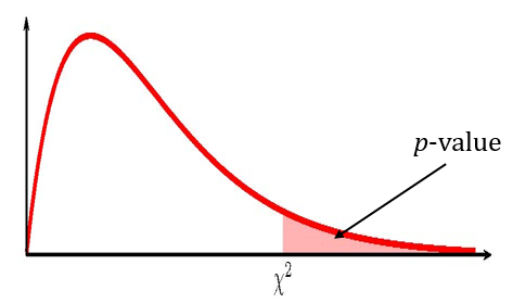
- Use the [latex]\chi^2[/latex]-distribution to find the [latex]p-\text{value}[/latex], which is the area in the right tail of the [latex]\chi^2[/latex]-distribution. The [latex]\chi^2[/latex]-score and degrees of freedom are
[latex]\begin{eqnarray*}\chi^2&=&\sum\frac{(\text{observed-expected})^2}{\text{expected}}\\\\df&=&k-1\\\\\text{observed}&=&\text{observed frequency from the sample data}\\\text{expected}&=&\text{expected frequency from assumed distribution}\\k&=&\text{number of categories}\\\\\end{eqnarray*}[/latex]
- Compare the [latex]p-\text{value}[/latex] to the significance level and state the outcome of the test.
- If [latex]p-\text{value}\leq\alpha[/latex], reject [latex]H_0[/latex] in favour of [latex]H_a[/latex].
- The results of the sample data are significant. There is sufficient evidence to conclude that the null hypothesis [latex]H_0[/latex] is an incorrect belief and that the alternative hypothesis [latex]H_a[/latex] is most likely correct.
- If [latex]p-\text{value}\gt\alpha[/latex], do not reject [latex]H_0[/latex].
- The results of the sample data are not significant. There is no sufficient evidence to conclude that the alternative hypothesis [latex]H_a[/latex] may be correct.
- If [latex]p-\text{value}\leq\alpha[/latex], reject [latex]H_0[/latex] in favour of [latex]H_a[/latex].
- Write down a concluding sentence specific to the context of the question.
NOTES
- The null hypothesis is the claim that the categorial variable follows the assumed distribution. That is, the probability [latex]p_i[/latex] of each possible outcome of the categorical variable equals a hypothesized probability [latex]p_{i_0}[/latex].
- The alternative hypothesis is the claim that the categorical variable does not follow the assumed distribution. That is, for at least one possible outcome of the categorical variable, the probability [latex]p_i[/latex] does not equal the claimed probability [latex]p_{i_0}[/latex].
- In order to use the [latex]\chi^2[/latex]-goodness-of-fit test, the expected frequency for each category must be at least [latex]5[/latex].
- The [latex]p-\text{value}[/latex] for a [latex]\chi^2[/latex]-goodness-of-fit test is always the area in the right tail of the [latex]\chi^2[/latex]-distribution. So, we use chisq.dist.rt to find the [latex]p-\text{value}[/latex] for a [latex]\chi^2[/latex]-goodness-of-fit test.
- To calculate the [latex]\chi^2[/latex]-score:
- For each of the possible outcomes of the categorical variable, calculate [latex]\displaystyle{\frac{(\text{observed-expected})^2}{\text{expected}}}[/latex]:
- Find the difference between the observed frequency (from the sample) and the expected frequency (from the null hypothesis). The expected frequency equals [latex]n\times p_{i_0}[/latex] where [latex]n[/latex] is the sample size and [latex]p_{i_0}[/latex] is the assumed probability for the [latex]i[/latex]th outcome claimed in the null hypothesis.
- Square the difference in step (i).
- Divide the value found in step (ii) by the expected frequency.
- Add up the values of [latex]\displaystyle{\frac{(\text{observed-expected})^2}{\text{expected}}}[/latex] for each of the outcomes.
- For each of the possible outcomes of the categorical variable, calculate [latex]\displaystyle{\frac{(\text{observed-expected})^2}{\text{expected}}}[/latex]:
- We expect that there will be a discrepancy between the observed frequency and the expected frequency. If this discrepancy is very large, the value of [latex]\chi^2[/latex] will be very large and result in a small [latex]p-\text{value}[/latex].
EXAMPLE
Absenteeism of college students from math classes is a major concern to math instructors because missing class appears to increase the drop rate. Suppose that a study was done to determine if the actual student absenteeism rate follows faculty perception. The faculty believe that the distribution of the number of absences per term is as follows:
| Number of Absences per Term | Expected Percent of Students |
|---|---|
| 0–2 | [latex]50\%[/latex] |
| 3–5 | [latex]30\%[/latex] |
| 6–8 | [latex]12\%[/latex] |
| 9–11 | [latex]6\%[/latex] |
| 12+ | [latex]2\%[/latex] |
At the end of the semester, a random survey of [latex]300[/latex] students across all mathematics courses was taken, and the actual (observed) number of absences for the [latex]300[/latex] students was recorded.
| Number of Absences per Term | Observed Number of Students |
|---|---|
| 0–2 | 120 |
| 3–5 | 100 |
| 6–8 | 55 |
| 9–11 | 15 |
| 12+ | 10 |
At the [latex]5\%[/latex] significance level, determine if the number of absences per term follows the distribution assumed by the faculty.
Solution
Let [latex]p_1[/latex] be the probability a student has 0-2 absences, [latex]p_2[/latex] be the probability a student has 3-5 absences, [latex]p_3[/latex] be the probability a student has 6-8 absences, [latex]p_4[/latex] be the probability a student has 9-11 absences, and [latex]p_5[/latex] be the probability a student has 12 or more absences.
Hypotheses:
[latex]\begin{eqnarray*}H_0:&&p_1=50\%,p_2=30\%,p_3=12\%,p_4=6\%,p_5=2\%\\H_a:&&\text{at least one of the }p_i's\text{ does not equal its stated probability}\end{eqnarray*}[/latex]
[latex]p-\text{value}[/latex]:
From the question, we have [latex]n=300[/latex] and [latex]k=5[/latex]. Now we need to calculate the [latex]\chi^2[/latex]-score for the test.
The observed frequency for each category is the number of observations in the sample that fall into that category. This is the information provided in the sample above.
Next, we must calculate out the expected frequencies. The expected frequency is the number of observations we would expect to see in the sample, assuming the null hypothesis is true. To calculate the expected frequency for each category, we multiply the sample size [latex]n[/latex] by the probability associated with that category claimed in the null hypothesis.
| Number of Absences per Term | Observed Frequency | Expected Frequency |
|---|---|---|
| 0-2 | 120 | 0.5[latex]\times[/latex]300=150 |
| 3-5 | 100 | 0.3[latex]\times[/latex]300=90 |
| 6-8 | 55 | 0.12[latex]\times[/latex]300=36 |
| 9-11 | 15 | 0.06[latex]\times[/latex]300=18 |
| 12+ | 10 | 0.02[latex]\times[/latex]300=6 |
To calculate the [latex]\chi^2[/latex]-score, we work out the quantity [latex]\displaystyle{\frac{(\text{observed-expected})^2}{\text{expected}}}[/latex] for each category and then add up these quantities.
[latex]\begin{eqnarray*}\chi^2&=&\sum\frac{(\text{observed-expected})^2}{\text{expected}}\\&=&\frac{(120-150)^2}{150}+\frac{(100-90)^2}{90}+\frac{(55-36)^2}{36}+\frac{(15-18)^2}{18}+\frac{(10-6)^2}{6}\\&=&20.305\ldots\end{eqnarray*}[/latex]
The degrees of freedom for the [latex]\chi^2[/latex]-distribution is [latex]df=k-1=5-1=4[/latex]. The [latex]\chi^2[/latex]-goodness-of-fit test is a right-tailed test, so we use the chisq.dist.rt function to find the [latex]p-\text{value}[/latex]:
| Function | chisq.dist.rt |
|---|---|
| Field 1 | 20.305.... |
| Field 2 | 4 |
| Answer | 0.0004 |
So the [latex]p-\text{value}=0.0004[/latex].
Conclusion:
Because [latex]p-\text{value}=0.0004\lt 0.05=\alpha[/latex], we reject the null hypothesis in favour of the alternative hypothesis. At the [latex]5\%[/latex] significance level, there is enough evidence to suggest that the number of absences per term does not follow the distribution assumed by faculty.
NOTES
- The null hypothesis is the claim that the percent of students that fall into each category is as stated. That is, [latex]50\%[/latex] students miss between 0 and 2 classes, [latex]30\%[/latex] of the students miss between 3 and 5 students, etc.
- The alternative hypothesis is the claim that at least one of the percent of students that fall into each category is not as stated. The alternative hypothesis does not say that every [latex]p_i[/latex] does not equal its stated probabilities, only that one of them does not equal its stated probability.
- Keep all of the decimals throughout the calculation (i.e. in the calculation of the [latex]\chi^2[/latex]-score) to avoid any round-off error in the calculation of the [latex]p-\text{value}[/latex]. This ensures that we get the most accurate value for the [latex]p-\text{value}[/latex]. Use Excel to calculate the expected frequencies and the [latex]\chi^2[/latex]-score.
- The [latex]p-\text{value}[/latex] is the area in the right tail of the [latex]\chi^2[/latex]-distribution, to the right of [latex]\chi^2=20.305...[/latex]. In the calculation of the [latex]p-\text{value}[/latex]:
- The function is chisq.dist.rt because we are finding the area in the right tail of a [latex]\chi^2[/latex]-distribution.
- Field 1 is the value of [latex]\chi^2[/latex].
- Field 2 is the value of the degrees of freedom [latex]df[/latex].
- The [latex]p-\text{value}[/latex] of [latex]0.0004[/latex] is a small probability compared to the significance level, and so is unlikely to happen assuming the null hypothesis is true. This suggests that the assumption that the null hypothesis is true is most likely incorrect, and so the conclusion of the test is to reject the null hypothesis in favour of the alternative hypothesis. In other words, student absenteeism does not fit faculty perception.
EXAMPLE
Employers want to know which days of the week employees have the highest number of absences in a five-day work week. Most employers would like to believe that employees are absent equally during the week. Suppose a random sample of [latex]60[/latex] managers are asked on which day of the week they had the highest number of employee absences. The results are recorded in the table below. At the [latex]5\%[/latex] significance level, test if the day of the week with the highest number of absences occurs with equal frequency during a five-day work week.
| Day of the Week | Observed Frequency |
|---|---|
| Monday | 15 |
| Tuesday | 11 |
| Wednesday | 10 |
| Thursday | 9 |
| Friday | 15 |
Solution
Let [latex]p_1[/latex] be the probability the highest number of absences occurs on Monday, [latex]p_2[/latex] be the probability the highest number of absences occurs on Tuesday, [latex]p_3[/latex] be the probability the highest number of absences occurs on Wednesday, [latex]p_4[/latex] be the probability the highest number of absences occurs on Thursday, and [latex]p_5[/latex] be the probability the highest number of absences occurs on Friday.
If the day of the week with the highest number of absences occurs with equal frequency, then the probability that any day has the highest number of absences is the same as any other day. Because there are [latex]5[/latex] days (categories), if the frequencies are equal, then each day would have a probability of [latex]20\%[/latex] [latex]\left(\text{or }\frac{1}{5}\right)[/latex].
Hypotheses:
[latex]\begin{eqnarray*}H_0:&&p_1=p_2=p_3=p_4=p_5=20\%\\H_a:&&\text{at least one of the }p_i\neq 20\%\end{eqnarray*}[/latex]
[latex]p-\text{value}[/latex]:
From the question, we have [latex]n=60[/latex] and [latex]k=5[/latex]. Now we need to calculate out the [latex]\chi^2[/latex]-score for the test.
The observed frequency for each category is the number of observations in the sample that fall into that category. This is the information provided in the sample above.
Next, we must calculate out the expected frequencies. The expected frequency is the number of observations we would expect to see in the sample, assuming the null hypothesis is true. To calculate the expected frequency for each category, we multiply the sample size [latex]n[/latex] by the probability associated with that category claimed in the null hypothesis.
| Day of the Week | Observed Frequency | Expected Frequency |
|---|---|---|
| Monday | 15 | 0.2[latex]\times[/latex]60=12 |
| Tuesday | 11 | 0.2[latex]\times[/latex]60=12 |
| Wednesday | 10 | 0.2[latex]\times[/latex]60=12 |
| Thursday | 9 | 0.2[latex]\times[/latex]60=12 |
| Friday | 15 | 0.2[latex]\times[/latex]60=12 |
To calculate the [latex]\chi^2[/latex]-score, we work out the quantity [latex]\displaystyle{\frac{(\text{observed-expected})^2}{\text{expected}}}[/latex] for each category and then add up these quantities.
[latex]\begin{eqnarray*}\chi^2&=&\sum\frac{(\text{observed-expected})^2}{\text{expected}}\\&=&\frac{(15-12)^2}{12}+\frac{(11-12)^2}{12}+\frac{(10-12)^2}{12}+\frac{(9-12)^2}{12}+\frac{(15-12)^2}{12}\\&=&2.666\ldots\end{eqnarray*}[/latex]
The degrees of freedom for the [latex]\chi^2[/latex]-distribution is [latex]df=k-1=5-1=4[/latex]. The [latex]\chi^2[/latex]-goodness-of-fit test is a right-tailed test, so we use the chisq.dist.rt function to find the [latex]p-\text{value}[/latex]:
| Function | chisq.dist.rt |
|---|---|
| Field 1 | 2.666.... |
| Field 2 | 4 |
| Answer | 0.6151 |
So the [latex]p-\text{value}=0.6151[/latex].
Conclusion:
Because [latex]p-\text{value}=0.6151\gt 0.05=\alpha[/latex], we do not reject the null hypothesis. At the [latex]5\%[/latex] significance level, there is enough evidence to suggest that the day of the week with the highest number of absences occurs with equal frequency during a five-day work week.
NOTES
- The null hypothesis is the claim that the probability each day of the week has the highest number of absences is [latex]20\%[/latex].
- The alternative hypothesis is the claim that at least one of the probabilities is not [latex]20\%[/latex]. The alternative hypothesis does not say that every [latex]p_i[/latex] does not equal [latex]20\%[/latex], only that one of them does not equal [latex]20\%[/latex].
- Keep all of the decimals throughout the calculation (i.e. in the calculation of the [latex]\chi^2[/latex]-score) to avoid any round-off error in the calculation of the [latex]p-\text{value}[/latex]. This ensures that we get the most accurate value for the [latex]p-\text{value}[/latex].
- The [latex]p-\text{value}[/latex] of [latex]0.6151[/latex] is a large probability compared to the significance level, and so is likely to happen assuming the null hypothesis is true. This suggests that the assumption that the null hypothesis is true is most likely correct, and so the conclusion of the test is to not reject the null hypothesis.
TRY IT
Teachers want to know which night each week their students are doing most of their homework. Most teachers think that students do an equal amount of homework each night. Suppose a random sample of [latex]49[/latex] students are asked on which night of the week they did the most homework. The results are shown in the table below. At the [latex]5\%[/latex] significance level, are the nights that students do most of their homework equally distributed?
| Day of Week | Number of Students |
|---|---|
| Sunday | 11 |
| Monday | 8 |
| Tuesday | 10 |
| Wednesday | 7 |
| Thursday | 10 |
| Friday | 5 |
| Saturday | 5 |
Click to see Solution
Let [latex]p_1[/latex] be the probability students do their homework on Sunday, [latex]p_2[/latex] be the probability students do their homework on Monday, [latex]p_3[/latex] be the probability students do their homework on Tuesday, [latex]p_4[/latex] be the probability students do their homework on Wednesday, [latex]p_5[/latex] be the probability students do their homework on Thursday, [latex]p_6[/latex] be the probability students do their homework on Friday, and [latex]p_7[/latex] be the probability students do their homework on Saturday.
Hypotheses:
[latex]\begin{eqnarray*}H_0:&&p_1=p_2=p_3=p_4=p_5=p_6=p_7=\frac{1}{7}\\H_a:&&\text{at least one of the }p_i\neq\frac{1}{7}\end{eqnarray*}[/latex]
[latex]p-\text{value}[/latex]:
From the question, we have [latex]n=49[/latex] and [latex]k=7[/latex].
| Day of the Week | Observed Frequency | Expected Frequency |
|---|---|---|
| Sunday | 11 | 1/7[latex]\times[/latex]49=7 |
| Monday | 8 | 1/7[latex]\times[/latex]49=7 |
| Tuesday | 10 | 1/7[latex]\times[/latex]49=7 |
| Wednesday | 7 | 1/7[latex]\times[/latex]49=7 |
| Thursday | 10 | 1/7[latex]\times[/latex]49=7 |
| Friday | 5 | 1/7[latex]\times[/latex]49=7 |
| Saturday | 5 | 1/7[latex]\times[/latex]49=7 |
[latex]\begin{eqnarray*}\chi^2&=&\sum\frac{(\text{observed-expected})^2}{\text{expected}}\\&=&\frac{(11-7)^2}{7}+\frac{(8-7)^2}{7}+\frac{(10-7)^2}{7}+\frac{(7-7)^2}{7}\\&&+\frac{(10-7)^2}{7}+\frac{(5-7)^2}{7}+\frac{(5-7)^2}{7}\\&=&6.142\ldots\end{eqnarray*}[/latex]
The degrees of freedom for the [latex]\chi^2[/latex]-distribution is [latex]df=k-1=7-1=6[/latex].
| Function | chisq.dist.rt |
|---|---|
| Field 1 | 6.142.... |
| Field 2 | 6 |
| Answer | 0.4074 |
So the [latex]p-\text{value}=0.4074[/latex].
Conclusion:
Because [latex]p-\text{value}=0.4074\gt 0.05=\alpha[/latex], we do not reject the null hypothesis. At the [latex]5\%[/latex] significance level, there is enough evidence to suggest that the nights students do most of their homework are equally distributed.
TRY IT
One study indicates that the number of televisions that American families have is distributed as shown in this table:
| Number of Televisions | Percent |
|---|---|
| 0 | [latex]10\%[/latex] |
| 1 | [latex]16\%[/latex] |
| 2 | [latex]55\%[/latex] |
| 3 | [latex]11\%[/latex] |
| 4 or more | [latex]8\%[/latex] |
A researcher wants to determine if the number of televisions that families in the far western part of the U.S. have the same distribution as the above study. A random sample of [latex]600[/latex] families in the far western U.S. is taken, and the results are recorded in the following table:
| Number of Televisions | Observed Frequency |
|---|---|
| 0 | 66 |
| 1 | 119 |
| 2 | 340 |
| 3 | 60 |
| 4 or more | 15 |
At the [latex]1\%[/latex] significance level, does it appear that the distribution of the number of televisions for families in the far western U.S is different from the distribution for the American population as a whole?
Click to see Solution
Let [latex]p_1[/latex] be the probability a family owns 0 televisions, [latex]p_2[/latex] be the probability a family owns 1 television, [latex]p_3[/latex] be the probability a family owns 2 televisions, [latex]p_4[/latex] be the probability a family owns 3 televisions, and [latex]p_5[/latex] be the probability a family owns 4 or more televisions.
Hypotheses:
[latex]\begin{eqnarray*}H_0:&&p_1=10\%,p_2=16\%,p_3=55\%,p_4=11\%,p_5=8\%\\H_a:&&\text{at least one of the }p_i's\text{ does not equal its stated probability}\end{eqnarray*}[/latex]
[latex]p-\text{value}[/latex]:
From the question, we have [latex]n=600[/latex] and [latex]k=5[/latex].
| Number of Televisions | Observed Frequency | Expected Frequency |
|---|---|---|
| 0 | 66 | 0.1[latex]\times[/latex]600=60 |
| 1 | 119 | 0.16[latex]\times[/latex]600=96 |
| 2 | 340 | 0.55[latex]\times[/latex]600=330 |
| 3 | 60 | 0.11[latex]\times[/latex]600=66 |
| 4 or more | 15 | 0.08[latex]\times[/latex]600=48 |
[latex]\begin{eqnarray*}\chi^2&=&\sum\frac{(\text{observed-expected})^2}{\text{expected}}\\&=&\frac{(66-60)^2}{60}+\frac{(119-96)^2}{96}+\frac{(340-330)^2}{330}+\frac{(60-66)^2}{66}+\frac{(15-48)^2}{48}\\&=&29.646\ldots\end{eqnarray*}[/latex]
The degrees of freedom for the [latex]\chi^2[/latex]-distribution is [latex]df=k-1=5-1=4[/latex].
| Function | chisq.dist.rt |
| Field 1 | 29.646.... |
| Field 2 | 4 |
| Answer | 0.000006 |
So the [latex]p-\text{value}=0.000006[/latex].
Conclusion:
Because [latex]p-\text{value}=0.000006\lt 0.01=\alpha[/latex], we reject the null hypothesis in favour of the alternative hypothesis. At the [latex]1\%[/latex] significance level, there is enough evidence to suggest that the distribution of the number of televisions for families in the far western U.S is different from the distribution for the American population as a whole.
TRY IT
The expected percentage of the number of pets students in the United States have in their homes is distributed as follows:
| Number of Pets | Percent |
|---|---|
| 0 | [latex]18\%[/latex] |
| 1 | [latex]25\%[/latex] |
| 2 | [latex]30\%[/latex] |
| 3 | [latex]18\%[/latex] |
| 4 or more | [latex]9\%[/latex] |
A researcher wants to find out if the distribution of the number of pets students in Canada have is the same as the distribution shown in the U.S. A random sample of [latex]1,000[/latex] students from Canada is taken, and the results are shown in the table below:
| Number of Pets | Observed Frequency |
|---|---|
| 0 | 210 |
| 1 | 240 |
| 2 | 320 |
| 3 | 140 |
| 4+ | 90 |
At the [latex]1\%[/latex] significance level, is the distribution of the number of pets students in Canada have different from the distribution for the United States?
Click to see Solution
Let [latex]p_1[/latex] be the probability a student owns 0 pets, [latex]p_2[/latex] be the probability a student owns 1 pet, [latex]p_3[/latex] be the probability a student owns 2 pets, [latex]p_4[/latex] be the probability a student owns 3 pets, and [latex]p_5[/latex] be the probability a student owns 4 or more pets.
Hypotheses:
[latex]\begin{eqnarray*}H_0:&&p_1=18\%,p_2=25\%,p_3=30\%,p_4=18\%,p_5=9\%\\H_a:&&\text{at least one of the }p_i's\text{ does not equal its stated probability}\end{eqnarray*}[/latex]
[latex]p-\text{value}[/latex]:
From the question, we have [latex]n=1000[/latex] and [latex]k=5[/latex].
| Number of Pets | Observed Frequency | Expected Frequency |
|---|---|---|
| 0 | 210 | 0.18[latex]\times[/latex]1000=180 |
| 1 | 240 | 0.25[latex]\times[/latex]1000=250 |
| 2 | 320 | 0.30[latex]\times[/latex]1000=300 |
| 3 | 140 | 0.18[latex]\times[/latex]1000=180 |
| 4 or more | 90 | 0.09[latex]\times[/latex]1000=90 |
[latex]\begin{eqnarray*}\chi^2&=&\sum\frac{(\text{observed-expected})^2}{\text{expected}}\\&=&\frac{(210-180)^2}{180}+\frac{(240-250)^2}{250}+\frac{(320-300)^2}{300}+\frac{(140-180)^2}{180}+\frac{(90-90)^2}{90}\\&=&15.622\ldots\end{eqnarray*}[/latex]
The degrees of freedom for the [latex]\chi^2[/latex]-distribution is [latex]df-k-1=5-1=4[/latex].
| Function | chisq.dist.rt |
|---|---|
| Field 1 | 15.622.... |
| Field 2 | 4 |
| Answer | 0.0036 |
So the [latex]p-\text{value}=0.0036[/latex].
Conclusion:
Because [latex]p-\text{value}=0.0036\lt 0.01=\alpha[/latex], we reject the null hypothesis in favour of the alternative hypothesis. At the [latex]1\%[/latex] significance level, there is enough evidence to suggest that the distribution of the number of pets students in Canada have is different from the distribution for the United States.
Video: "Pearson's chi square test (goodness of fit) | Probability and Statistics | Khan Academy" by Khan Academy [11:48] is licensed under the Standard YouTube License.Transcript and closed captions available on YouTube.
Exercises
- A teacher predicts that the distribution of grades on the final exam will be as follows:
Grade Percent A [latex]25\%[/latex] B [latex]30\%[/latex] C [latex]35\%[/latex] D [latex]10\%[/latex] In a class of [latex]20[/latex] students, the frequency of the grades on the final exam is given below:
Grade Frequency A 7 B 7 C 5 D 1 At the [latex]5\%[/latex] significance level, do the actual grades match the teacher's assumed distribution?
Click to see Answer
- Hypotheses: [latex]\begin{eqnarray*}H_0:&&p_1=25\%,p_2=30\%,p_3=35\%,p_4=10\%\\H_a:&&\text{at least one of the }p_i's\text{ does not equal its stated probability}\end{eqnarray*}[/latex]
- [latex]p-\text{value}=0.5645[/latex]
- Conclusion: At the [latex]5\%[/latex] significance level, there is enough evidence to conclude that the distribution of grades on the final exam follows the teacher's stated distribution.
- A six-sided die is rolled [latex]120[/latex] times, and the results are recorded in the table below. At the [latex]5\%[/latex] significance level, determine if the die is fair. (Hint: in a fair die, each of the faces is equally likely to occur.)
Face Value Frequency 1 15 2 29 3 16 4 15 5 30 6 15 Click to see Answer
- Hypotheses: [latex]\begin{eqnarray*}H_0:&&p_1=p_2=p_3=p_4=p_5=p_6=16.67\%\\H_a:&&\text{at least one of the }p_i's\text{ does not equal }16.67\%\end{eqnarray*}[/latex]
- [latex]p-\text{value}=0.0184[/latex]
- Conclusion: At the [latex]5\%[/latex] significance level, there is enough evidence to conclude that the distribution of the dice rolls does not follow the assumed distribution. The dice is not fair.
- The distribution of the marital status for the male population of certain country, ages 15 and older, is as shown in the table below.
Marital Status Percent never married [latex]31.3\%[/latex] married [latex]56.1\%[/latex] widowed [latex]2.5\%[/latex] divorced/separated [latex]10.1\%[/latex] Suppose that a random sample of [latex]400[/latex] young adult males from the country, ages 18 to 24 years old, yield the following frequency distribution.
Marital Status Frequency never married 140 married 238 widowed 2 divorced/separated 20 At the [latex]1\%[/latex] significance level, test if this young adult male age group fits the distribution of the adult male population of the country.
Click to see Answer
- Hypotheses: [latex]\begin{eqnarray*}H_0:&&p_1=31.3\%,p_2=56.1\%,p_3=2.5\%,p_4=10.1\%\\H_a:&&\text{at least one of the }p_i's\text{ does not equal its stated probability}\end{eqnarray*}[/latex]
- [latex]p-\text{value}=0.0002[/latex]
- Conclusion: At the [latex]1\%[/latex] significance level, there is enough evidence to conclude that the distribution of the martial statues of the young adult male age group is different than the distribution of the adult male population.
- The columns in the table below contain the Race/Ethnicity of the high schools in a certain country for a recent year and the percentages of the Overall Student Population. A local school district wants to determine if its high schools follow the same distribution for the ethnicity of its students. The school district takes a sample of [latex]1,000[/latex] high school students in the district, and the right column in the table contains the breakdown of the ethnicity of the students in the sample.
Race/Ethnicity Overall Student Population Survey Frequency Asian, Asian American, or Pacific Islander [latex]5.4\%[/latex] 82 Black [latex]14.5\%[/latex] 135 Hispanic or Latino [latex]15.9%[/latex] 136 Indigenous [latex]1.2\%[/latex] 10 White [latex]61.6\%[/latex] 604 Not reported/other [latex]1.4\%[/latex] 33 At the [latex]5\%[/latex] significance level, determine if the distribution of ethnicity at the local school district follows the overall student population.
Click to see Answer
- Hypotheses: [latex]\begin{eqnarray*}H_0:&&p_1=5.4\%,p_2=14.5\%,p_3=15.9\%,p_4=1.2\%,p_5=61.6\%,p_6=1.4\%\\H_a:&&\text{at least one of the }p_i's\text{ does not equal its stated probability}\end{eqnarray*}[/latex]
- [latex]p-\text{value}=0.0018[/latex]
- Conclusion: At the [latex]5\%[/latex] significance level, there is enough evidence to conclude that the distribution of the ethnicity of high schools in the local district is different than the distribution of the overall high school student population.
- The table below shows the expected distribution of majors of all male university students across the country. A local university wants to know if the distribution of majors for its male students follows the same distribution. A sample of [latex]5,000[/latex] male students at the university is taken, and their majors are recorded. The data from the sample is shown in the right column in the table.
Major Expected Major Actual Major Arts & Humanities [latex]12.0\%[/latex] 630 Biological Sciences [latex]6.7\%[/latex] 320 Business [latex]22.7\%[/latex] 1100 Education [latex]5.8\%[/latex] 315 Engineering [latex]15.6\%[/latex] 800 Physical Sciences [latex]3.6\%[/latex] 175 Professional [latex]9.3\%[/latex] 450 Social Sciences [latex]7.6\%[/latex] 370 Technical [latex]1.8\%[/latex] 90 Other [latex]8.2\%[/latex] 400 Undecided [latex]6.7\%[/latex] 350 At the [latex]5\%[/latex] significance level, determine if the distribution of the majors of male students at the local university fits the distribution of majors for all male university students.
Click to see Answer
- Hypotheses: [latex]\begin{align*}&H_0:p_1=12\%,p_2=6.7\%,p_3=22.7\%,p_4=5.8\%,p_5=15.6\%,p_6=3.6\%,p_7=9.3\%,p_8=7.6\%,p_9=1.8\%,p_{10}=8.2\%,p_{11}=6.7\%\\&H_a:\text{at least one of the }p_i's\text{ does not equal its stated probability}\end{align*}[/latex]
- [latex]p-\text{value}=0.6561[/latex]
- Conclusion: At the [latex]5\%[/latex] significance level, there is enough evidence to conclude that the distribution of majors for male students at the local university follows the distribution of majors for all male university students across the country.
- The table below shows the expected distribution of majors of all female university students across the country. A local university wants to know if the distribution of majors for its female students follows the same distribution. A sample of [latex]5,000[/latex] female students at the university is taken, and their majors are recorded. The data from the sample is shown in the right column in the table.
Major Expected Major Actual Major Arts & Humanities [latex]14.0\%[/latex] 670 Biological Sciences [latex]8.4\%[/latex] 410 Business [latex]13.1\%[/latex] 685 Education [latex]13.0\%[/latex] 650 Engineering [latex]2.6\%[/latex] 145 Physical Sciences [latex]2.6\%[/latex] 125 Professional [latex]18.9\%[/latex] 975 Social Sciences [latex]13.0\%[/latex] 605 Technical [latex]0.4\%[/latex] 15 Other [latex]5.8\%[/latex] 300 Undecided [latex]8.2\%[/latex] 420 At the [latex]5\%[/latex] significance level, determine if the distribution of majors of female students at the local university fits the distribution of majors for all female university students.
Click to see Answer
- Hypotheses:[latex]\begin{eqnarray*}H_0:&&p_1=14\%,p_2=8.4\%,p_3=13.1\%,p_4=13\%,p_5=2.6\%,p_6=2.6\%,p_7=18.9\%,p_8=13\%,p_9=0.4\%,p_{10}=5.8\%,p_{11}=8.2\%\\H_a:&&\text{at least one of the }p_i's\text{ does not equal its stated probability}\end{eqnarray*}[/latex]
- [latex]p-\text{value}=0.3791[/latex]
- Conclusion: At the [latex]5\%[/latex] significance level, there is enough evidence to conclude that the distribution of majors for female students at the local university follows the distribution of majors for all female university students across the country.
- A local police department wants to know if the percentage of traffic accidents is the same for each day of the week. The department takes a sample of [latex]500[/latex] traffic accidents and records the day of the week on which they occurred.
Day of the Week Frequency Sunday 75 Monday 60 Tuesday 74 Wednesday 57 Thursday 65 Friday 79 Saturday 90 At the [latex]5\%[/latex] significance level, determine if the proportion of traffic accidents is the same for each day of the week.
Click to see Answer
- Hypotheses:[latex]\begin{eqnarray*}H_0:&&p_1=p_2=p_3=p_4=p_5=p_6=p_7=14.29\%\\H_a:&&\text{at least one of the }p_i's\text{ does not equal }14.29\%\end{eqnarray*}[/latex]
- [latex]p-\text{value}=0.0817[/latex]
- Conclusion: At the [latex]5\%[/latex] significance level, there is enough evidence to conclude that the proportion of traffic accidents is the same for each day of the week.
- A local retailer provides a variety of payment options for its customers: cash, cheque, credit and debit. The retailer believes that the current distribution of the payment options is as follows: [latex]15\%[/latex] cash, [latex]5\%[/latex] cheque, [latex]50\%[/latex] credit, and [latex]30\%[/latex] debit. The retailer takes a sample of [latex]450[/latex] transactions and records the payment method
Payment Method Frequency Cash 78 Cheque 12 Credit 250 Debit 110 At the [latex]1\%[/latex] significance level, determine if the retailer's claimed distribution of the payment methods is correct.
Click to see Answer
- Hypotheses:[latex]\begin{eqnarray*}H_0:&&p_1=15\%,p_2=5\%,p_3=50\%,p_4=30\%\\H_a:&&\text{at least one of the }p_i's\text{ does not equal its stated probability}\end{eqnarray*}[/latex]
- [latex]p-\text{value}=0.003[/latex]
- Conclusion: At the [latex]1\%[/latex] significance level, there is enough evidence to conclude that the distribution of the payment methods is different than the retailer's claim.
- A local restaurant owner has five locations across the city. The owner wants to know if the percentage of customers is the same at each location. The owner takes a sample of [latex]750[/latex] customers and records which restaurant location they visited.
Location Frequency 1 126 2 179 3 141 4 131 5 173 At the [latex]1\%[/latex] significance level, determine if the proportion of customers is the same for each restaurant location.
Click to see Answer
- Hypotheses:[latex]\begin{eqnarray*}H_0:&&p_1=p_2=p_3=p_4=p_5=20\%\\H_a:&&\text{at least one of the }p_i's\text{ does not equal }20\%\end{eqnarray*}[/latex]
- [latex]p-\text{value}=0.0031[/latex]
- Conclusion: At the [latex]1\%[/latex] significance level, there is enough evidence to conclude that the proportion of customers is not the same for each location.
"10.4 The Goodness-of-Fit Test" and “10.6 Exercises” from Introduction to Statistics by Valerie Watts is licensed under a Creative Commons Attribution-NonCommercial-ShareAlike 4.0 International License, except where otherwise noted.
