10.2 Statistical Inference for a Single Population Variance
LEARNING OBJECTIVES
- Calculate and interpret a confidence interval for a population variance.
- Conduct and interpret a hypothesis test on a single population variance.
The mean of a population is important, but in many cases, the variance of the population is just as important. In most production processes, quality is measured by how closely the process matches the target (i.e. the mean) and by the variability (i.e. the variance) of the process. For example, if a process is to fill bags of coffee beans, we are interested in both the mean weight of the bag and how much variation there is in the weight of the bags. The quality is considered poor if the mean weight of the bags is accurate, but the variance of the weight of the bags is too high—a variance that is too large means some bags would be too full, and some bags would be almost empty.
As with other population parameters, we can construct a confidence interval to capture the population variance and conduct a hypothesis test on the population variance. In order to construct a confidence interval or conduct a hypothesis test on a population variance [latex]\sigma^2[/latex], we need to use the distribution of [latex]\displaystyle{\frac{(n-1)\times s^2}{\sigma^2}}[/latex]. Suppose we have a normal population with population variance [latex]\sigma^2[/latex], and a sample of size [latex]n[/latex] is taken from the population. The sampling distribution of [latex]\displaystyle{\frac{(n-1)\times s^2}{\sigma^2}}[/latex] follows a [latex]\chi^2[/latex]-distribution with [latex]n-1[/latex] degrees of freedom.
Constructing a Confidence Interval for a Population Variance
To construct the confidence interval, take a random sample of size [latex]n[/latex] from a normally distributed population. Calculate the sample variance [latex]s^2[/latex]. The limits for the confidence interval with confidence level [latex]C[/latex] for an unknown population variance [latex]\sigma^2[/latex] are
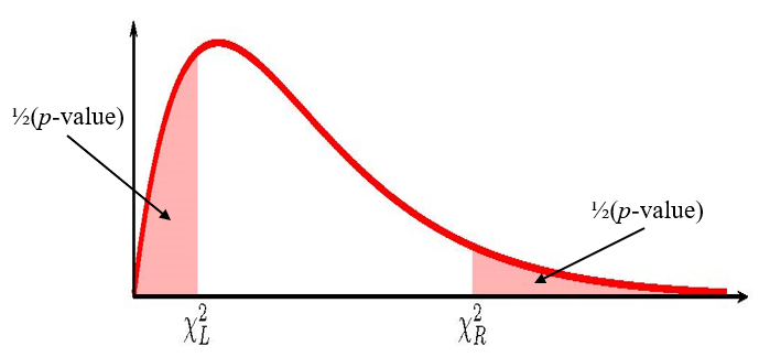
[latex]\begin{eqnarray*}\text{Lower Limit}&=&\frac{(n-1)\times s^2}{\chi^2_R}\\\\\text{Upper Limit}&=&\frac{(n-1)\times s^2}{\chi^2_L}\\\\\end{eqnarray*}[/latex]
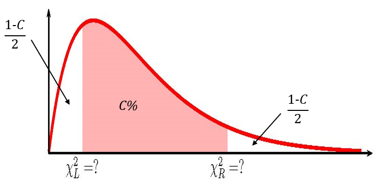
where [latex]\chi^2_L[/latex] is the [latex]\chi^2[/latex]-score so that the area in the left tail of the [latex]\chi^2[/latex]-distribution is [latex]\displaystyle{\frac{1-C}{2}}[/latex], [latex]\chi^2_R[/latex] is the [latex]\chi^2[/latex]-score so that the area in the right tail of the [latex]\chi^2[/latex]-distribution is [latex]\displaystyle{\frac{1-C}{2}}[/latex] and the [latex]\chi^2[/latex]-distribution has [latex]n-1[/latex] degrees of freedom.
NOTES
- Like the other confidence intervals we have seen, the [latex]\chi^2[/latex]-scores are the values that trap [latex]C\%[/latex] of the observations in the middle of the distribution so that the area of each tail is [latex]\displaystyle{\frac{1-C}{2}}[/latex].
- Because the [latex]\chi^2[/latex]-distribution is not symmetrical, the confidence interval for a population variance requires that we calculate two different [latex]\chi^2[/latex]-scores: one for the left tail and one for the right tail. In Excel, we need to use both the chisq.inv function (for the left tail) and the chisq.inv.rt function (for the right tail) to find the two different [latex]\chi^2[/latex]-scores.
- The [latex]\chi^2[/latex]-score for the left tail is part of the formula for the upper limit, and the [latex]\chi^2[/latex]-score for the right tail is part of the formula for the lower limit. This is not a mistake. It follows from the formula used to determine the limits for the confidence interval.
EXAMPLE
A local telecom company conducts broadband speed tests to measure how much data per second passes between a customer's computer and the internet compared to what the customer pays for as part of their plan. The company needs to estimate the variance in the broadband speed. A sample of [latex]15[/latex] ISPs is taken, and the amount of data per second is recorded. The variance in the sample is [latex]174[/latex].
- Construct a [latex]97\%[/latex] confidence interval for the variance in the amount of data per second that passes between a customer's computer and the internet.
- Interpret the confidence interval found in part 1.
Solution
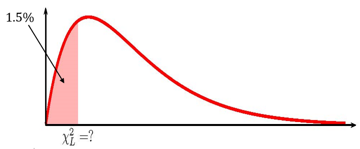
- To find the confidence interval, we need to find the [latex]\chi^2_L[/latex]-score for the [latex]97\%[/latex] confidence interval. This means that we need to find the [latex]\chi^2_L[/latex]-score so that the area in the left tail is [latex]\displaystyle{\frac{1-0.97}{2}=0.015}[/latex]. The degrees of freedom for the [latex]\chi^2[/latex]-distribution is [latex]n-1=15-1=14[/latex].
| Function | chisq.inv |
|---|---|
| Field 1 | 0.015 |
| Field 2 | 14 |
| Answer | 5.0572... |
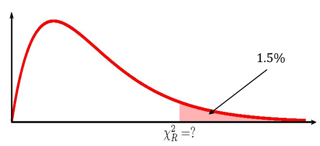
We also need to find the [latex]\chi^2_R[/latex]-score for the [latex]97\%[/latex] confidence interval. This means that we need to find the [latex]\chi^2_R[/latex]-score so that the area in the right tail is [latex]\displaystyle{\frac{1-0.97}{2}=0.015}[/latex]. The degrees of freedom for the [latex]\chi^2[/latex]-distribution is [latex]n-1=15-1=14[/latex].
| Function | chisq.inv.rt |
|---|---|
| Field 1 | 0.015 |
| Field 2 | 14 |
| Answer | 27.826... |
So [latex]\chi^2_L=5.0572\ldots[/latex] and [latex]\chi^2_R=27.826\ldots[/latex]. From the sample data supplied in the question [latex]s^2=174[/latex] and [latex]n=15[/latex]. The [latex]97\%[/latex] confidence interval is
[latex]\begin{eqnarray*}\text{Lower Limit}&=&\frac{(n-1)\times s^2}{\chi^2_R}\\&=&\frac{(15-1)\times 174}{27.826\ldots}\\&=&87.54\\\\\text{Upper Limit}&=&\frac{(n-1)\times s^2}{\chi^2_R}\\&=&\frac{(15-1)\times 174}{5.0572\ldots}\\&=&481.69\\\\\end{eqnarray*}[/latex]
- We are [latex]97\%[/latex] confident that the variance in the amount of data per second that passes between a customer's computer and the internet is between [latex]87.54[/latex] and [latex]481.69[/latex].
NOTES
- When calculating the limits for the confidence interval, keep all of the decimals in the [latex]\chi^2[/latex]-scores and other values throughout the calculation. This will ensure that there is no round-off error in the answer. Use Excel to do the calculations of the limits, clicking on the cells containing the [latex]\chi^2[/latex]-scores and any other values.
- When writing down the interpretation of the confidence interval, make sure to include the confidence level and the actual population variance captured by the confidence interval (i.e. be specific to the context of the question).
TRY IT
A pharmaceutical company manufactures a particular drug. To ensure that patients receive the proper dose, the variance in the weight of the drug is critical. The company's quality control department routinely assesses the drug as it is produced to ensure it meets production guidelines. From the latest production run, a sample of [latex]40[/latex] units of the drug is taken, and the weight, in grams, of each unit is recorded. The variance of the weights is [latex]0.27[/latex]
- Construct a [latex]95\%[/latex] confidence interval for the variance in the weight of the drug.
- Interpret the confidence interval found in part 1.
- If the variance in the weight of the drug exceeds [latex]0.5[/latex], the drug is rejected. Based on the sample, should the quality control department reject the latest production run of the drug? Explain.
Click to see Solution
-
Function chisq.inv Field 1 0.025 Field 2 39 Answer 23.654... Function chisq.inv.rt Field 1 0.025 Field 2 39 Answer 58.120... [latex]\begin{eqnarray*}\text{Lower Limit}&=&\frac{(n-1)\times s^2}{\chi^2_R}\\&=&\frac{(40-1)\times 0.27}{58.120\ldots}\\&=&0.181\\\\\text{Upper Limit}&=&\frac{(n-1)\times s^2}{\chi^2_R}\\&=&\frac{(40-1)\times 0.27}{23.654\ldots}\\&=&0.445\\\\\end{eqnarray*}[/latex]
- We are [latex]95\%[/latex] confident that the variance in the weight of the drug is between [latex]0.181[/latex] and [latex]0.445[/latex].
- The quality control department should not reject the latest production run of the drug because [latex]0.5[/latex] is outside the confidence interval. The variance of the weight of the drug does not exceed [latex]0.5[/latex].
Conducting a Hypothesis Test for a Population Variance
Follow these steps to perform a hypothesis test for a population variance:
- Write down the null and alternative hypotheses in terms of the population variance [latex]\sigma^2[/latex].
- Use the form of the alternative hypothesis to determine if the test is left-tailed, right-tailed, or two-tailed.
- Collect the sample information for the test and identify the significance level [latex]\alpha[/latex].
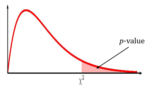
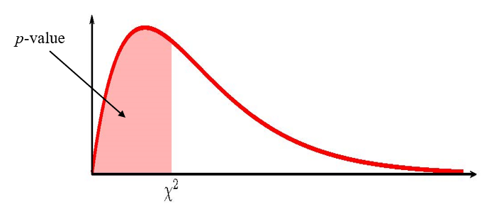
- Use the [latex]\chi^2[/latex]-distribution to find the [latex]p-\text{value}[/latex] (the area in the corresponding tail) for the test. The [latex]\chi^2[/latex]-score and degrees of freedom are
[latex]\begin{eqnarray*}\chi^2=\frac{(n-1)\times s^2}{\sigma^2}&\;\;\;\;\;\;\;\;&df=n-1\\\\\end{eqnarray*}[/latex]
- Compare the [latex]p-\text{value}[/latex] to the significance level and state the outcome of the test.
- If [latex]p-\text{value}\leq\alpha[/latex], reject [latex]H_0[/latex] in favour of [latex]H_a[/latex].
- The results of the sample data are significant. There is sufficient evidence to conclude that the null hypothesis [latex]H_0[/latex] is an incorrect belief and that the alternative hypothesis [latex]H_a[/latex] is most likely correct.
- If [latex]p-\text{value}\gt\alpha[/latex], do not reject [latex]H_0[/latex].
- The results of the sample data are not significant. There is insufficient evidence to conclude that the alternative hypothesis [latex]H_a[/latex] may be correct.
- If [latex]p-\text{value}\leq\alpha[/latex], reject [latex]H_0[/latex] in favour of [latex]H_a[/latex].
- Write down a concluding sentence specific to the context of the question.
EXAMPLE
A statistics instructor at a local college claims that the variance for the final exam scores was [latex]25[/latex]. After speaking with his classmates, one of the class's best students thinks that the variance for the final exam scores is higher than the instructor claims. The student challenges the instructor to prove her claim. The instructor takes a sample [latex]30[/latex] final exams and finds the variance of the scores is [latex]28[/latex]. At the [latex]5\%[/latex] significance level, test if the variance of the final exam scores is higher than the instructor claims.
Solution
Hypotheses:
[latex]\begin{eqnarray*}H_0:&&\sigma^2=25\\H_a:&&\sigma^2\gt 25\end{eqnarray*}[/latex]
[latex]p-\text{value}[/latex]:
From the question, we have [latex]n=30[/latex], [latex]s^2=28[/latex], and [latex]\alpha=0.05[/latex].
Because the alternative hypothesis is a [latex]\gt[/latex], the [latex]p\text{-value}[/latex] is the area in the right tail of the [latex]\chi^2[/latex]-distribution.
To use the chisq.dist.rt function, we need to calculate out the [latex]\chi^2[/latex]-score and the degrees of freedom:
[latex]\begin{eqnarray*}\chi^2&=&\frac{(n-1)\times s^2}{\sigma^2}\\&=&\frac{(30-1)\times 28}{25}\\&=&32.48\\\\df&=&n-1\\&=&30-1\\&=&29\end{eqnarray*}[/latex]
| Function | chisq.dist.rt |
|---|---|
| Field 1 | 32.48 |
| Field 2 | 29 |
| Answer | 0.2992 |
So the [latex]p-\text{value}=0.2992[/latex].
Conclusion:
Because [latex]p-\text{value}=0.2992\gt 0.05=\alpha[/latex], we do not reject the null hypothesis. At the [latex]5\%[/latex] significance level, there is not enough evidence to suggest that the variance of the final exam scores is higher than [latex]25[/latex].
NOTES
- The null hypothesis [latex]\sigma^2=25[/latex] is the claim that the variance on the final exam is [latex]25[/latex].
- The alternative hypothesis [latex]\sigma^2\gt 25[/latex] is the claim that the variance on the final exam is greater than [latex]25[/latex].
- The [latex]p-\text{value}[/latex] is the area in the right tail of the [latex]\chi^2[/latex]-distribution, to the right of [latex]\chi^2=32.84[/latex]. In the calculation of the [latex]p-\text{value}[/latex]:
- The function is chisq.dist.rt because we are finding the area in the right tail of a [latex]\chi^2[/latex]-distribution.
- Field 1 is the value of [latex]\chi^2[/latex].
- Field 2 is the degrees of freedom.
- The [latex]p-\text{value}[/latex] of [latex]0.2992[/latex] is a large probability compared to the significance level and so is likely to happen, assuming the null hypothesis is true. This suggests that the assumption that the null hypothesis is true is most likely correct, and so the conclusion of the test is to not reject the null hypothesis. In other words, the variance of the scores on the final exam is most likely [latex]25[/latex].
EXAMPLE
With individual lines at its various windows, a post office finds that the standard deviation for normally distributed waiting times for customers is [latex]7.2[/latex] minutes. The post office experiments with a single, main waiting line and finds that for a random sample of [latex]25[/latex] customers, the waiting times for customers have a standard deviation of [latex]4.5[/latex] minutes. At the [latex]5\%[/latex] significance level, determine if the single line changed the variation among the wait times for customers.
Solution
Hypotheses:
[latex]\begin{eqnarray*}H_0:&&\sigma^2=51.84\\H_a:&&\sigma^2\neq 51.84\end{eqnarray*}[/latex]
[latex]p-\text{value}[/latex]:
From the question, we have [latex]n=25[/latex], [latex]s^2=20.25[/latex], and [latex]\alpha=0.05[/latex].
Because the alternative hypothesis is a [latex]\neq[/latex], the [latex]p-\text{value}[/latex] is the sum of the areas in the tails of the [latex]\chi^2[/latex]-distribution.
We need to calculate out the [latex]\chi^2[/latex]-score and the degrees of freedom:
[latex]\begin{eqnarray*}\chi^2&=&\frac{(n-1)\times s^2}{\sigma^2}\\&=&\frac{(25-1)\times 20.25}{51.84}\\&=&9.375\\\\df&=&n-1\\&=&25-1\\&=&24\end{eqnarray*}[/latex]
Because this is a two-tailed test, we need to know which tail (left or right) the [latex]\chi^2[/latex]-score belongs to so that we can use the correct Excel function. If [latex]\chi^2\gt df-2[/latex], the [latex]\chi^2[/latex]-score corresponds to the right tail. If the [latex]\chi^2\lt df-2[/latex], the [latex]\chi^2[/latex]-score corresponds to the left tail. In this case, [latex]\chi^2=9.375\lt 22=df-2[/latex], so the [latex]\chi^2[/latex]-score corresponds to the left tail. We need to use chisq.dist to find the area in the left tail.
| Function | chisq.dist |
| Field 1 | 9.375 |
| Field 2 | 24 |
| Answer | 0.0033 |
So the area in the left tail is [latex]0.0033[/latex], which means that [latex]\frac{1}{2}(p-\text{value})=0.0033[/latex]. This is also the area in the right tail, so
[latex]p-\text{value}=0.0033+0.0033=0.0066[/latex]
Conclusion:
Because [latex]p-\text{value}=0.0066\lt 0.05=\alpha[/latex], we reject the null hypothesis in favour of the alternative hypothesis. At the [latex]5\%[/latex] significance level, there is enough evidence to suggest that the variation among the wait times for customers has changed.
NOTES
- The null hypothesis [latex]\sigma^2=51.84[/latex] is the claim that the variance in the wait times is [latex]51.84[/latex]. Note that we were given the standard deviation ([latex]\sigma=7.2[/latex]) in the question. But this is a test on variance, so we must write the hypotheses in terms of the variance [latex]\sigma^2=7.2^2=51.84[/latex].
- The alternative hypothesis [latex]\sigma^2\neq 51.84[/latex] is the claim that the variance in the wait times has changed from [latex]51.84[/latex].
- In a two-tailed hypothesis test for population variance, we will only have sample information relating to one of the two tails. We must determine which of the tails the sample information belongs to, and then calculate out the area in that tail. The area in each tail represents exactly half of the [latex]p-\text{value}[/latex], so the [latex]p-\text{value}[/latex] is the sum of the areas in the two tails.
- If [latex]\chi^2\lt df-2[/latex], the sample information belongs to the left tail.
- We use chisq.dist to find the area in the left tail. The area in the right tail equals the area in the left tail, so we can find the [latex]p-\text{value}[/latex] by adding the output from this function to itself.
- If [latex]\chi^2\gt df-2[/latex], the sample information belongs to the right tail.
- We use chisq.dist.rt to find the area in the right tail. The area in the left tail equals the area in the right tail, so we can find the [latex]p-\text{value}[/latex] by adding the output from this function to itself.
- If [latex]\chi^2\lt df-2[/latex], the sample information belongs to the left tail.
- The [latex]p-\text{value}[/latex] of [latex]0.0066[/latex] is a small probability compared to the significance level and so is unlikely to happen assuming the null hypothesis is true. This suggests that the assumption that the null hypothesis is true is most likely incorrect, and so the conclusion of the test is to reject the null hypothesis in favour of the alternative hypothesis. In other words, the variance in the wait times has most likely changed.
TRY IT
A scuba instructor wants to record the collective depths each of his students dives during their checkout. He is interested in how the depths vary, even though everyone should have been at the same depth. He believes the standard deviation of the depths is [latex]1.2[/latex] meters. But his assistant thinks the standard deviation is less than [latex]1.2[/latex] meters. The instructor wants to test this claim. The scuba instructor uses his most recent class of [latex]20[/latex] students as a sample and finds that the standard deviation of the depths is [latex]0.85[/latex] meters. At the [latex]1\%[/latex] significance level, test if the variability in the depths of the student scuba divers is less than claimed.
Click to see Solution
Hypotheses:
[latex]\begin{eqnarray*}H_0:&&\sigma^2=1.44\\H_a:&&\sigma^2\lt 1.44\end{eqnarray*}[/latex]
[latex]p-\text{value}[/latex]:
From the question, we have [latex]n=20[/latex], [latex]s^2=0.7225[/latex], and [latex]\alpha=0.01[/latex].
Because the alternative hypothesis is a [latex]\lt[/latex], the [latex]p-\text{value}[/latex] is the area in the left tail of the [latex]\chi^2[/latex]-distribution.
To use the chisq.dist function, we need to calculate out the [latex]\chi^2[/latex]-score and the degrees of freedom:
[latex]\begin{eqnarray*}\chi^2&=&\frac{(n-1)\times s^2}{\sigma^2}\\&=&\frac{(20-1)\times 0.7225}{1.44}\\&=&9.5329\ldots\\\\df&=&n-1\\&=&20-1\\&=&19\end{eqnarray*}[/latex]
| Function | chisq.dist |
| Field 1 | 9.5329... |
| Field 2 | 19 |
| Field 3 | true |
| Answer | 0.0365 |
So the [latex]p-\text{value}=0.0365[/latex].
Conclusion:
Because [latex]p-\text{value}=0.0365\gt 0.01=\alpha[/latex], we do not reject the null hypothesis. At the [latex]1\%[/latex] significance level, there is not enough evidence to suggest that the variation in the depths of the students is less than claimed.
Video: "Hypothesis Tests for One Population Variance" by jbstatistics [8:52] is licensed under the Standard YouTube License.Transcript and closed captions available on YouTube.
Exercises
- An archer claims that the variance for his hits is [latex]36[/latex] (data is measured in distance from the center of the target). An observer claims the archer's standard deviation for his hits is less, and the observer wants to test her claim at the [latex]5\%[/latex] significance level. The observer takes a sample of [latex]30[/latex] of the archer's hits and finds a variance of [latex]29.16[/latex].
Click to see Answer
- Hypotheses: [latex]\begin{eqnarray*}H_0:&&\sigma^2=36\\H_a:&&\sigma^2\lt 36\end{eqnarray*}[/latex]
- [latex]p-\text{value}=0.2463[/latex]
- Conclusion: At the [latex]5\%[/latex] significance level, there is not enough evidence to conclude that the archer's variance is less than [latex]36[/latex].
- In the past, the variance of heights for students in a school is [latex]0.66[/latex]. A researcher believes the variation of the heights of students at the school is greater than [latex]0.66[/latex]. A random sample of [latex]50[/latex] students at the school is taken, and the standard deviation of heights in the sample is [latex]0.96[/latex]. At the [latex]5\%[/latex] significance level, determine if the variance in the heights for students in the school is greater than [latex]0.66[/latex].
Click to see Answer
- Hypotheses: [latex]\begin{eqnarray*}H_0:&&\sigma^2=0.66\\H_a:&&\sigma^2\gt 0.66\end{eqnarray*}[/latex]
- [latex]p-\text{value}=0.0347[/latex]
- Conclusion: At the [latex]5\%[/latex] significance level,l there is enough evidence to conclude that the variation in student heights at the school is greater than [latex]0.66[/latex].
- The average waiting time to see a doctor at a medical clinic varies. One doctor at the clinic wants to estimate the variance in the waiting times. In a random sample of [latex]30[/latex] patients at the medical clinic, the standard deviation of waiting times of [latex]4.1[/latex] minutes.
- Construct a [latex]96\%[/latex] confidence interval for the variation in the wait times at the doctor's office.
- Interpret the confidence interval found in part (a).
- The doctor investigating the variance of wait times believes that the variance in the wait times is greater than [latex]12[/latex]. Is the doctor's claim reasonable? Explain.
Click to see Answer
- [latex]\text{Lower Limit}=10.44[/latex], [latex]\text{Upper Limit}=31.30[/latex]
- There is a [latex]96\%[/latex] probability that the variance in the weight times is between [latex]10.44[/latex] and [latex]31.30[/latex].
- Yes, because [latex]12[/latex] is inside the confidence interval.
- Suppose an airline claims that its flights are consistently on time with an average delay of at most [latex]15[/latex] minutes. It claims that the average delay is so consistent that the variance is no more than [latex]150[/latex]. Doubting the consistency part of the claim, a disgruntled traveller calculates the delays for his next [latex]25[/latex] flights. The average delay for those [latex]25[/latex] flights is [latex]22[/latex] minutes with a standard deviation of [latex]15[/latex] minutes. At the [latex]5\%[/latex] significance level, determine if the variance in the delay times is greater than [latex]150[/latex].
Click to see Answer
- Hypotheses: [latex]\begin{eqnarray*}H_0:&&\sigma^2=150\\H_a:&&\sigma^2\gt 150\end{eqnarray*}[/latex]
- [latex]p-\text{value}=0.0853[/latex]
- Conclusion: At the [latex]5\%[/latex] significance level, there is not enough evidence to conclude that the variance in the delay times is greater than [latex]150[/latex].
- A plant manager at a cereal production company is concerned her equipment may need recalibrating. It seems that the actual weight of the [latex]750[/latex] gram cereal boxes the equipment fills has been fluctuating. In order to determine if the machine needs to be recalibrated, [latex]84[/latex] randomly selected boxes of cereal from the next day’s production were weighed. The variance of the [latex]84[/latex] boxes was [latex]1.3[/latex].
- Construct a [latex]98\%[/latex] confidence interval for the variance in the weight of the cereal boxes.
- Interpret the confidence interval found in part (a).
- If the variance in the weight of the cereal boxes is supposed to be at most [latex]2[/latex], does the machine need to be recalibrated?
Click to see Answer
- [latex]\text{Lower Limit}=0.931[/latex], [latex]\text{Upper Limit}=1.927[/latex]
- There is a [latex]98\%[/latex] probability that the variance in the weight of the cereal boxes is between [latex]0.931[/latex] and [latex]1.927[/latex].
- No, because [latex]2[/latex] is outside the confidence interval.
- Consumers may be interested in whether the cost of a particular calculator varies from store to store. A major retailer claims that the variation in the price of the calculator is [latex]225[/latex]. But one consumer doubts this claim and believes that the variance in the price of the calculator is greater than [latex]225[/latex]. Based on a sample of [latex]43[/latex] stores, the consumer found that the mean price of the calculator was [latex]\$84[/latex] and a standard deviation of [latex]\$18[/latex]. At the [latex]5\%[/latex] significance level, test the consumer's claim that the variance in the price of the calculator is greater than [latex]225[/latex].
Click to see Answer
- Hypotheses: [latex]\begin{eqnarray*}H_0:&&\sigma^2=225\\H_a:&&\sigma^2\gt 225\end{eqnarray*}[/latex]
- [latex]p-\text{value}=0.0322[/latex]
- Conclusion: At the [latex]5\%[/latex] significance level, there is enough evidence to conclude that the variance in the price of the calculator is greater than [latex]225[/latex].
- Airline companies are interested in the consistency of the number of babies on each flight so that they have adequate safety equipment. They are also interested in the variation of the number of babies. Suppose that an airline executive believes the variance in the number of babies per flight is [latex]9[/latex]. The airline wants to test the executive's claim to see if the variance is different than claimed. The airline takes a sample of [latex]18[/latex] flights and finds that the standard deviation for the number of babies per flight is [latex]4.1[/latex]. Conduct a hypothesis test of the airline executive’s belief. Use a [latex]1\%[/latex] significance level.
Click to see Answer
- Hypotheses: [latex]\begin{eqnarray*}H_0:&&\sigma^2=9\\H_a:&&\sigma^2\neq 9\end{eqnarray*}[/latex]
- [latex]p-\text{value}=0.0323[/latex]
- Conclusion: At the [latex]1\%[/latex] significance level, there is not enough evidence to conclude that the variance in the number of babies per flight is different from [latex]9[/latex].
- According to an avid aquarist, the variance for the number of fish in a 20-gallon tank is [latex]4[/latex]. His friend, also an aquarist, does not believe this claim and that the variance is actually different from [latex]4[/latex]. She counts the number of fish in [latex]15[/latex] other 20-gallon tanks and gets the following results:
11 11 11 9 11 10 10 10 7 10 9 10 12 9 11 At the [latex]5\%[/latex] significance level, test the claim that the variance for the number of fish in a 20-gallon tank is different than [latex]4[/latex].
Click to see Answer
- Hypotheses: [latex]\begin{eqnarray*}H_0:&&\sigma^2=4\\H_a:&&\sigma^2\neq 4\end{eqnarray*}[/latex]
- [latex]p-\text{value}=0.0354[/latex]
- Conclusion: At the [latex]5\%[/latex] significance level, there is enough evidence to conclude that the variance in the number of fish in a 20-gallon tank is different from [latex]4[/latex].
- The manager of "Frenchies" is concerned that patrons are not consistently receiving the same amount of French fries with each order. The chef claims that the variation for an order of fries is [latex]2.25[/latex], but the manager thinks that it may be lower. He randomly weighs [latex]49[/latex] orders of fries, which yields a variance of [latex]1.49[/latex]. At the [latex]1\%[/latex] significance level, determine if the variation in the amount of fries per order is less than claimed.
Click to see Answer
- Hypotheses: [latex]\begin{eqnarray*}H_0:&&\sigma^2=2.25\\H_a:&&\sigma^2\lt 2.25\end{eqnarray*}[/latex]
- [latex]p-\text{value}=0.0344[/latex]
- Conclusion: At the [latex]1\%[/latex] significance level, there is not enough evidence to conclude that the variance in the amount of fries per order is less than [latex]2.25[/latex].
- You want to buy a specific computer. A sales representative of the manufacturer claims that retail stores sell this computer at an average price of [latex]\$1,249[/latex] with a variance of [latex]625[/latex]. You find a website that has a price comparison for the same computer at a series of stores as follows:
$1299 $1299.99 $1193.08 $1279 1224.95 1229.99 1269.95 1249 Can you argue that the variation in the price of the computer is different than what is claimed by the manufacturer? Use the [latex]5\%[/latex] significance level.
Click to see Answer
- Hypotheses: [latex]\begin{eqnarray*}H_0:&&\sigma^2=625\\H_a:&&\sigma^2\neq 625\end{eqnarray*}[/latex]
- [latex]p-\text{value}=0.0459[/latex]
- Conclusion: At the [latex]5\%[/latex] significance level, there is enough evidence to conclude that the variance in the price of the computer is greater than [latex]625[/latex].
- A company packages apples by weight. One of the weight grades is Class A apples. A batch of apples is selected to be included in a Class A apple package. The weights of the selected apples (in grams) is as follows:
158 167 149 169 164 139 154 150 157 171 152 161 141 166 172 - Construct a [latex]95\%[/latex] confidence interval for the variation in the weight of apples in the package.
- Interpret the confidence interval found in part (a).
Click to see Answer
- [latex]\text{Lower Limit}=58.35[/latex], [latex]\text{Upper Limit}=270.75[/latex]
- There is a [latex]95\%[/latex] probability that the variance in the weight of the apples is between [latex]58.35[/latex] and [latex]270.75[/latex].
"10.3 Statistical Inference for a Single Population Variance" and “10.6 Exercises” from Introduction to Statistics by Valerie Watts is licensed under a Creative Commons Attribution-NonCommercial-ShareAlike 4.0 International License, except where otherwise noted.
