9.4 Statistical Inference for Two Population Proportions

Valerie Watts

9.4 Statistical Inference for Two Population Proportions

LEARNING OBJECTIVES

Construct and interpret a confidence interval for two population proportions.
Conduct and interpret hypothesis tests for two population proportions.

Similar to comparing two population means, the comparison of two population proportions is very common. Often, we want to find out if the two populations under study have the same proportion or if there is some difference in the two population proportions. Unlike two population means, we can only approach the comparison of two population proportions using independent samples. Recall that two populations are independent if the sample taken from population 1 is not related in any way to the sample taken from population 2. In this situation, any relationship between the samples or populations is entirely coincidental.

Throughout this section, we will use subscripts to identify the values for the proportions and sample sizes for the two populations:

Symbol for:

Population 1

Population 2

Population Proportion

[latex]p_1[/latex]

[latex]p_2[/latex]

Sample Size

[latex]n_1[/latex]

[latex]n_2[/latex]

Sample Proportion

[latex]\hat{p}_1[/latex]

[latex]\hat{p}_2[/latex]

Number of Items in Sample with Characteristic of Interest

[latex]x_1[/latex]

[latex]x_2[/latex]

In order to construct a confidence interval or conduct a hypothesis test on the difference in two population proportions ([latex]p_1-p_2[/latex]), we need to use the distribution of the difference in the sample proportions [latex]\hat{p}_1-\hat{p}_2[/latex].

The mean of the distribution of the difference in the sample proportions is [latex]\displaystyle{\mu_{\hat{p}_1-\hat{p}_2}}=p_1-p_2[/latex].
The standard deviation of the distribution of the difference in the sample proportions is [latex]\displaystyle{\sigma_{\hat{p}_1-\hat{p}_2}=\sqrt{\frac{p_1\times(1-p_1)}{n_1}+\frac{p_2\times(1-p_2)}{n_2}}}[/latex].
The distribution of the difference in the sample proportions is normal if [latex]n_1\times p_1\geq 5[/latex], [latex]n_1\times(1-p_1)\geq 5[/latex], [latex]n_2 \times p_2 \geq 5[/latex] and [latex]n_2\times(1-p_2)\geq 5[/latex].
Assuming the distribution of the difference of the sample proportions is normal, the [latex]z[/latex]-score is [latex]\displaystyle{z=\frac{(\hat{p}_1-\hat{p}_2)-(p_1-p_2)}{\sqrt{\frac{p_1\times(1-p_1)}{n_1}+\frac{p_2\times(1-p_2)}{n_2}}}}[/latex].

Constructing a Confidence Interval for the Difference in Two Population Proportions

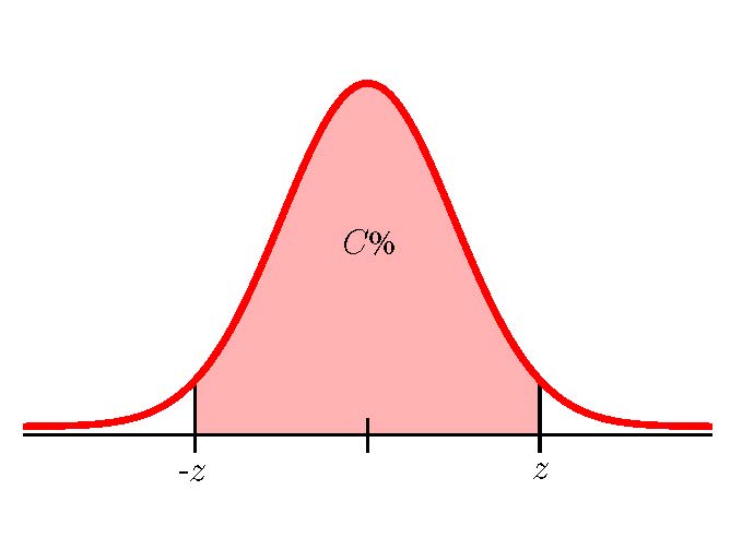
Suppose a sample of size [latex]n_1[/latex] with sample proportion [latex]\hat{p}_1[/latex] is taken from population 1 and a sample of size [latex]n_2[/latex] with sample proportion [latex]\hat{p}_2[/latex] is taken from population 2. The limits for the confidence interval with confidence level [latex]C[/latex] for the difference in the population proportions [latex]\displaystyle{p_1-p_2}[/latex] are

[latex]\begin{eqnarray*}\\\text{Lower Limit}&=&\hat{p}_1-\hat{p}_2-z\times\sqrt{\frac{\hat{p}_1\times(1-\hat{p}_1)}{n_1}+\frac{\hat{p_2}\times(1-\hat{p}_2)}{n_2}}\\\\\text{Upper Limit}&=&\hat{p}_1-\hat{p}_2+z\times\sqrt{\frac{\hat{p}_1\times(1-\hat{p}_1)}{n_1}+\frac{\hat{p_2}\times(1-\hat{p}_2)}{n_2}}\\\\\end{eqnarray*}[/latex]

where [latex]z[/latex] is the [latex]z[/latex]-score of the standard normal distribution so that the area to the left of [latex]z[/latex] is [latex]\displaystyle{C+\frac{1-C}{2}}[/latex].

NOTES

In order to construct the confidence interval for the difference in two population proportions, we need to check that the normal distribution applies. This means that we need to check that [latex]n_1\times p_1\geq 5[/latex], [latex]n_1\times(1-p_1)\geq 5[/latex], [latex]n_2 \times p_2 \geq 5[/latex] and [latex]n_2\times(1-p_2)\geq 5[/latex].
Because the population proportions [latex]p_1[/latex] and [latex]p_2[/latex] are often unknown, we replace the values of the population proportions with the sample proportions [latex]\hat{p}_1[/latex] and [latex]\hat{p}_2[/latex] in the normal distribution check. That is, when the population proportions are unknown, we check [latex]n_1\times\hat{p}_1\geq 5[/latex], [latex]n_1 \times (1-\hat{p}_1) \geq 5[/latex], [latex]n_2\times\hat{p}_2\geq 5[/latex] and [latex]n_2\times(1-\hat{p}_2)\geq 5[/latex] to verify that the normal distribution applies.

CALCULATING THE [latex]{\color{white}{z}}[/latex]-SCORE FOR A CONFIDENCE INTERVAL IN EXCEL

To find the [latex]z[/latex]-score to construct a confidence interval with confidence level [latex]C[/latex], use the norm.s.inv(area to the left of z) function.

For area to the left of z, enter the entire area to the left of the [latex]z[/latex]-score you are trying to find. For a confidence interval, the area to the left of [latex]z[/latex] is [latex]\displaystyle{C+\frac{1-C}{2}}[/latex].

The output from the norm.s.inv function is the value of the [latex]z[/latex]-score needed to construct the confidence interval.

NOTE

The norm.s.inv function requires that we enter the entire area to the left of the unknown [latex]z[/latex]-score. This area includes the confidence level [latex]C[/latex] (the area in the middle of the distribution) plus the remaining area in the left tail [latex]\frac{1-C}{2}[/latex].

EXAMPLE

A marketing company places an advertisement for a new brand of deodorant on two different platforms: television and social media. The company wants to study the proportion of people who remembered seeing the advertisement two hours later. In a sample of [latex]200[/latex] people who saw the advertisement on television, [latex]74[/latex] remembered seeing it two hours later. In a sample of [latex]300[/latex] people who saw the advertisement on social media, [latex]129[/latex] remembered seeing it two hours later.

Construct a [latex]98\%[/latex] confidence interval for the difference in the proportion of people from the two different platforms that remember seeing the advertisement two hours later.
Interpret the confidence interval found in part 1.
Is there evidence to suggest that the proportion of people from social media who remember seeing the advertisement two hours later is greater than the proportion of people from television? Explain.

Solution

Let television be population 1 and social media be population 2. From the question, we have the following information:

Television Social Media

[latex]n_1=200[/latex] [latex]n_2=300[/latex]

[latex]\hat{p}_1=\frac{74}{200}=0.37[/latex] [latex]\hat{p}_2=\frac{129}{300}=0.43[/latex]

Before constructing the confidence interval, we check that the normal distribution applies:

[latex]\begin{eqnarray*}n_1\times\hat{p}_1&=&200\times 0.37=74\geq 5\\n_1\times(1-\hat{p}_1)&=&200\times(1-0.37)=126\geq 5\\n_2\times\hat{p}_2&=&300\times 0.43=129\geq 5\\n_2\times(1-\hat{p}_1)&=&300\times(1-0.37)=171\geq 5\end{eqnarray*}[/latex]

To find the confidence interval, we need to find the [latex]z[/latex]-score for the [latex]98\%[/latex] confidence interval. This means that we need to find the [latex]z[/latex]-score so that the entire area to the left of [latex]z[/latex] is [latex]\displaystyle{0.98+\frac{1-0.98}{2}=0.99}[/latex].

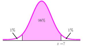
Function norm.s.inv

Field 1 0.99

Answer 2.3263…

So [latex]z=2.3263...[/latex]. The [latex]98\%[/latex] confidence interval is

[latex]\begin{eqnarray*}\\\text{Lower Limit}&=&\hat{p}_1-\hat{p}_2-z\times\sqrt{\frac{\hat{p}_1\times(1-\hat{p}_1)}{n_1}+\frac{\hat{p_2}\times(1-\hat{p}_2)}{n_2}}\\&=&0.37-0.43-2.3263...\times\sqrt{\frac{0.37\times(1-0.37)}{200}+\frac{0.43\times(1-0.43)}{300}}\\&=&-0.1636\\\\\text{Upper Limit}&=&\hat{p}_1-\hat{p}_2+z\times\sqrt{\frac{\hat{p}_1\times(1-\hat{p}_1)}{n_1}+\frac{\hat{p_2}\times(1-\hat{p}_2)}{n_2}}\\&=&0.37-0.43+2.3263...\times\sqrt{\frac{0.37\times(1-0.37)}{200}+\frac{0.43\times(1-0.43)}{300}}\\&=&0.0436\\\\\end{eqnarray*}[/latex]
We are [latex]98\%[/latex] confident that the difference in the proportion of people from the two platforms that remember seeing the advertisement two hours later is between [latex]-16.36%[/latex] and [latex]4.36\%[/latex].
Because [latex]0[/latex] is inside the confidence interval, it suggests that the difference in the proportions [latex]\displaystyle{p_1-p_2}[/latex] is [latex]0[/latex]. That is, [latex]\displaystyle{p_1-p_2=0}[/latex]. This suggests that the two proportions are equal. So the proportion of people from social media who remember seeing the advertisement two hours is not greater than the proportion of people from television.

NOTES

Because the population proportions are unknown, we use the sample proportions in the check for normality.
When calculating the limits for the confidence interval, keep all of the decimals in the [latex]z[/latex]-score and other values throughout the calculation. This will ensure that there is no round-off error in the answers. Use Excel to do the calculation of the limits, clicking on the cell containing the [latex]z[/latex]-score and any other values, to ensure that all of the decimal places are used in the calculation.
The limits for the confidence interval are percents. For example, the upper limit of [latex]0.0436[/latex] is the decimal form of a percent: [latex]4.36\%[/latex].
When writing down the interpretation of the confidence interval, make sure to include the confidence level, the actual difference in the population proportions captured by the confidence interval (i.e. be specific to the context of the question), and express the limits as percents.

Conducting a Hypothesis Test for the Difference in Two Population Proportions

Follow these steps to perform a hypothesis test on the difference in two population proportions:

Write down the null hypothesis that there is no difference in the population proportions:
[latex]\begin{eqnarray*}\\H_0:&&p_1-p_2=0\end{eqnarray*}[/latex]

The null hypothesis is always the claim that the two population proportions are equal ([latex]p_1=p_2[/latex]).
Write down the alternative hypotheses in terms of the difference in the population proportions. The alternative hypothesis will be one of the following:
[latex]\begin{eqnarray*}H_a:p_1-p_2<0&&(p_1\lt p_2)\\H_a:p_1-p_2>0&&(p_1\gt p_2)\\H_a:p_1-p_2\neq 0&&(p_1\neq p_2)\\\\\end{eqnarray*}[/latex]
Use the form of the alternative hypothesis to determine if the test is left-tailed, right-tailed, or two-tailed.
Collect the sample information for the test and identify the significance level.
Check the conditions [latex]n_1\times\hat{p}_1\geq 5[/latex], [latex]n_1 \times (1-\hat{p}_1) \geq 5[/latex], [latex]n_2\times\hat{p}_2\geq 5[/latex] and [latex]n_2\times(1-\hat{p}_2)\geq 5[/latex] to verify that the normal distribution applies. Use the normal distribution to find the [latex]p-\text{value}[/latex] (the area in the corresponding tail) for the test. The [latex]z[/latex]-score is
[latex]\begin{eqnarray*}z=\frac{(\hat{p}_1-\hat{p}_2)-(p_1-p_2)}{\sqrt{\overline{p}\times(1-\overline{p})\times\left(\frac{1}{n_1}+\frac{1}{n_2}\right)}}&\;\;\;\;\;\;\;\;\;\;\;\;&\overline{p}=\frac{x_1+x_2}{n_1+n_2}\\\\\end{eqnarray*}[/latex]
Compare the [latex]p-\text{value}[/latex] to the significance level and state the outcome of the test.
- If [latex]p-\text{value}\leq\alpha[/latex], reject [latex]H_0[/latex] in favour of [latex]H_a[/latex].
  - The results of the sample data are significant. There is sufficient evidence to conclude that the null hypothesis [latex]H_0[/latex] is an incorrect belief and that the alternative hypothesis [latex]H_a[/latex] is most likely correct.
- If [latex]p-\text{value}\gt\alpha[/latex], do not reject [latex]H_0[/latex].
  - The results of the sample data are not significant. There is not sufficient evidence to conclude that the alternative hypothesis [latex]H_a[/latex] may be correct.
Write down a concluding sentence specific to the context of the question.

NOTES

Because the population proportions [latex]p_1[/latex] and [latex]p_2[/latex] are often unknown, we replace the values of the population proportions with the sample proportions [latex]\hat{p}_1[/latex] and [latex]\hat{p}_2[/latex] in the normal distribution check. That is, when the population proportions are unknown, we check [latex]n_1\times\hat{p}_1\geq 5[/latex], [latex]n_1 \times (1-\hat{p}_1) \geq 5[/latex], [latex]n_2\times\hat{p}_2\geq 5[/latex] and [latex]n_2\times(1-\hat{p}_2)\geq 5[/latex] to verify that the normal distribution applies to the calculation of the p-value.
Because we are testing the equality of the two population proportions, the [latex]z[/latex]-score for the hypothesis test uses a pooled sample proportion [latex]\overline{p}[/latex]. The pooled sample proportion [latex]\overline{p}[/latex] combines the sample data to create an estimate of the overall proportion of success.

USING EXCEL TO CALCULE THE [latex]{\color{white}{p-\text{value}}}[/latex] FOR A HYPOTHESIS TEST ON TWO INDEPENDENT POPULATION PROPORTIONS

The [latex]p-\text{value}[/latex] for a hypothesis test on the difference in two population proportions is the area in the tail(s) of the normal distribution, assuming that the conditions for using a normal distribution are met ([latex]n_1\times p_1\geq 5[/latex], [latex]n_1\times(1-p_1)\geq 5[/latex], [latex]n_2 \times p_2 \geq 5[/latex] and [latex]n_2\times(1-p_2)\geq 5[/latex] ).

The [latex]p-\text{value}[/latex] is the area in the tail(s) of a normal distribution, so the norm.dist(x,[latex]\mu[/latex],[latex]\sigma[/latex],logic operator) function can be used to calculate the [latex]p-\text{value}[/latex].

For x, enter the value for [latex]\hat{p}_1-\hat{p}_2[/latex].
For [latex]\mu[/latex], enter [latex]0[/latex], the value of [latex]p_1-p_2[/latex] from the null hypothesis. This is the mean of the distribution of the differences in the sample proportions.
For [latex]\sigma[/latex], enter the value of [latex]\displaystyle{\sqrt{\overline{p}\times(1-\overline{p})\times\left(\frac{1}{n_1}+\frac{1}{n_2}\right)}}[/latex] where [latex]\displaystyle{\overline{p}=\frac{x_1+x_2}{n_1+n_2}}[/latex]. The value for [latex]\sigma[/latex] is the bottom part of the [latex]z[/latex]-score used in the hypothesis test.
For the logic operator, enter true. Note: Because we are calculating the area under the curve, we always enter true for the logic operator.

As with the previous chapter, use the appropriate technique with the norm.dist function to find the area in the left-tail, the area in the right-tail or the sum of the area in tails.

EXAMPLE

A cell phone company claimed that iPhones are more popular with adults 30 years old or younger than with adults over 30 years old. A consumer advocacy group wants to test this claim. In a sample of [latex]1340[/latex] adults 30 years old or younger, [latex]134[/latex] own an iPhone. In a sample of [latex]250[/latex] adults over the age of 30, [latex]15[/latex] own an iPhone. At the [latex]5\%[/latex] significance level, is the proportion of adults 30 years old or younger who own an iPhone greater than the proportion of adults over the age of 30 who own an iPhone?

Solution

Let adults 30 years old or younger be population 1 and adults over 30 years old be population 2. From the question, we have the following information:

30 Years or Younger

Over 30 Years

[latex]n_1=1340[/latex]

[latex]n_2=250[/latex]

[latex]x_1=134[/latex]

[latex]x_2=15[/latex]

[latex]\hat{p}_1=\frac{134}{1340}=0.1[/latex]

[latex]\hat{p}_2=\frac{15}{250}=0.05[/latex]

Hypotheses:

[latex]\begin{eqnarray*}H_0:&&p_1-p_2=0\\H_a:&&p_1-p_2\gt 0\end{eqnarray*}[/latex]

[latex]p-\text{value}[/latex]:

Before calculating the [latex]p-\text{value}[/latex], we check that the normal distribution applies:

[latex]\begin{eqnarray*}n_1\times\hat{p}_1&=&1340\times 0.1=134\geq 5\\n_1\times(1-\hat{p}_1)&=&1340\times(1-0.1)=1206\geq 5\\n_2\times\hat{p}_2&=&250\times 0.05=15\geq 5\\n_2\times(1-\hat{p}_1)&=&250\times(1-0.05)=235\geq 5\end{eqnarray*}[/latex]

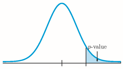
Because [latex]n_1 \times \hat{p}_1 \geq 5[/latex], [latex]n_1\times(1-\hat{p}_1)\geq 5[/latex], [latex]n_2 \times \hat{p}_2 \geq 5[/latex], and [latex]n_2\times(1-\hat{p}_2)\geq 5[/latex], the normal distribution applies, and so we use a normal distribution to calculate the [latex]p-\text{value}[/latex]. Because the alternative hypothesis is a [latex]\gt[/latex], the [latex]p-\text{value}[/latex] is the area in the right tail of the distribution.

The pooled sample proportion is:

[latex]\begin{eqnarray*}\overline{p}&=&\frac{x_1+x_2}{n_1+n_2}\\&=&\frac{134+15}{1340+250}\\&=&\frac{149}{1590}\\&=&0.09371\ldots\end{eqnarray*}[/latex]

Function

1-norm.dist

Field 1

0.1-0.05

Field 2

0

Field 3

sqrt(0.09371… *(1-0.09371…)*(1/1340+1/250))

Field 4

true

Answer

0.0232

So the [latex]p-\text{value}=0.0232[/latex].

Conclusion:

Because [latex]p-\text{value}=0.0232\lt 0.05=\alpha[/latex], we reject the null hypothesis in favour of the alternative hypothesis. At the [latex]5\%[/latex] significance level there is enough evidence to suggest that the proportion of adults 30 years old or younger who own an iPhone is greater than the proportion of adults over the age of 30 who own an iPhone.

NOTES

The null hypothesis [latex]p_1-p_2=0[/latex] is the claim that the proportion of adults 30 or younger with an iPhone equals the proportion of adults over 30 with an iPhone ([latex]p_1=p_2[/latex]). That is, the two populations have the same proportion.
The alternative hypothesis [latex]p_1-p_2\gt 0[/latex] is the claim that the proportion of adults 30 or younger with an iPhone is greater than the proportion of adults over 30 with an iPhone ([latex]p_1\gt p_2[/latex]).
Make sure to keep all of the decimal places throughout the calculation to avoid any round-off error in the [latex]p-\text{value}[/latex]. Perform the calculations of the sample proportions and the pooled sample proportion [latex]\overline{p}[/latex] in Excel and then click on the corresponding cells when completing the fields in the norm.dist function.
The [latex]p-\text{value}[/latex] is the area in the right tail of the normal distribution. In the calculation of the [latex]p-\text{value}[/latex]:
- The function is 1-norm.dist because we are finding the area in the right tail of a normal distribution.
- Field 1 is the value of [latex]\hat{p}_1-\hat{p}_2=0.1-0.05[/latex].
- Field 2 is [latex]0[/latex], the value of [latex]p_1-p_2[/latex] from the null hypothesis. Remember, we run the test assuming the null hypothesis is true, so that means we assume [latex]p_1-p_2=0[/latex].
- Field 3 is the value of
  [latex]\small\sqrt{\overline{p}\times(1-\overline{p})\times\left(\frac{1}{n_1}+\frac{1}{n_2}\right)}=\sqrt{0.09371\ldots\times(1-0.09371\ldots)\times\left(\frac{1}{1340}+\frac{1}{250}\right)}[/latex]
The [latex]p-\text{value}[/latex] of [latex]0.0232[/latex] is a small probability compared to the significance level, and so is unlikely to happen assuming that the null hypothesis is true. This suggests that the assumption that the null hypothesis is true is most likely incorrect, and so the conclusion of the test is to reject the null hypothesis in favour of the alternative hypothesis. In other words, the proportion of adults 30 years old or younger who own an iPhone is greater than the proportion of adults over the age of 30 who own an iPhone.

EXAMPLE

Two types of medication for hives are tested to determine if there is a difference in the proportions of adult patient reactions. In a sample of [latex]200[/latex] adults given medication A, [latex]20[/latex] still had hives 30 minutes after taking the medication. In a sample of [latex]200[/latex] adults given medication B, [latex]12[/latex] still had hives 30 minutes after taking the medication. At the [latex]1\%[/latex] significance level, is there a difference in the proportion of adults who still have hives 30 minutes after taking medications?

Solution

Let medication A be population 1 and medication B be population 2. From the question, we have the following information:

Medication A

Medication B

[latex]n_1=200[/latex]

[latex]n_2=200[/latex]

[latex]x_1=20[/latex]

[latex]x_2=12[/latex]

[latex]\hat{p}_1=\frac{20}{200}=0.1[/latex]

[latex]\hat{p}_2=\frac{12}{200}=0.06[/latex]

Hypotheses:

[latex]\begin{eqnarray*}H_0:&&p_1-p_2=0\\H_a:&&p_1-p_2\neq 0\end{eqnarray*}[/latex]

[latex]p-\text{value}[/latex]:

Before calculating the [latex]p-\text{value}[/latex], we check that the normal distribution applies:

[latex]\begin{eqnarray*}n_1\times\hat{p}_1&=&200\times 0.1=20\geq 5\\n_1\times(1-\hat{p}_1)&=&200\times(1-0.1)=180\geq 5\\n_2\times\hat{p}_2&=&200\times 0.06=12\geq 5\\n_2\times(1-\hat{p}_1)&=&200\times(1-0.06)=188\geq 5\end{eqnarray*}[/latex]

Because [latex]n_1 \times \hat{p}_1 \geq 5[/latex], [latex]n_1\times(1-\hat{p}_1)\geq 5[/latex], [latex]n_2 \times \hat{p}_2 \geq 5[/latex], and [latex]n_2\times(1-\hat{p}_2)\geq 5[/latex], the normal distribution applies, and so we use a normal distribution to calculate the [latex]p-\text{value}[/latex]. Because the alternative hypothesis is a [latex]\neq[/latex], the [latex]p-\text{value}[/latex] is the sum of the area in the two tails of the distribution.

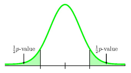
We need to know if the sample information relates to the left or right tail because that will determine how we calculate out the area of that tail using the normal distribution. In this case, [latex]\hat{p}_1\gt\hat{p}_2[/latex] ([latex]0.1\gt 0.06[/latex]), so the sample information relates to the right tail of the normal distribution. This means that we will calculate out the area in the right tail using 1-norm.dist. However, this is a two-tailed test where the [latex]p-\text{value}[/latex] is the sum of the area in the two tails, and the area in the right tail is only one-half of the [latex]p-\text{value}[/latex]. The area in the right tail equals the area in the left tail, and the [latex]p-\text{value}[/latex] is the sum of these two areas.

The pooled sample proportion is:

[latex]\begin{eqnarray*}\overline{p}&=&\frac{x_1+x_2}{n_1+n_2}\\&=&\frac{20+12}{200+200}\\&=&\frac{32}{400}\\&=&0.08\end{eqnarray*}[/latex]

Function

1-norm.dist

Field 1

0.1-0.06

Field 2

0

Field 3

sqrt(0.08*(1-0.08)*(1/200+1/200))

Field 4

true

Answer

0.0702

So the area in the right tail is [latex]0.0702[/latex], which means [latex]\frac{1}{2}p-\text{value}=0.0702[/latex]. This is also the area in the left tail, so

[latex]p-\text{value}=0.0702+0.0702=0.1404[/latex]

Conclusion:

Because [latex]p-\text{value}=0.1404\gt 0.01=\alpha[/latex], we do not reject the null hypothesis. At the [latex]1\%[/latex] significance level, there is not enough evidence to suggest that there is a difference in the proportion of adults who still have hives 30 minutes after taking medication.

NOTES

The null hypothesis [latex]p_1-p_2=0[/latex] is the claim that there is no difference in the proportion of adults with hives 30 minutes after taking the medications ([latex]p_1=p_2[/latex]). That is, the two populations have the same proportion.
The alternative hypothesis [latex]p_1-p_2\neq 0[/latex] is the claim that there is a difference in the proportion of adults with hives 30 minutes after taking the medications ([latex]p_1\neq p_2[/latex]).
Make sure to keep all of the decimal places throughout the calculation to avoid any round-off error in the [latex]p-\text{value}[/latex]. Perform the calculations of the sample proportions and the pooled sample proportion [latex]\overline{p}[/latex] in Excel and then click on the corresponding cells when completing the fields in the norm.dist function.
In a two-tailed hypothesis test that uses the normal distribution, we will only have sample information relating to one of the two tails. We must determine which of the tails the sample information belongs to and then calculate out the area in that tail. The area in each tail represents exactly half of the [latex]p-\text{value}[/latex], so the [latex]p-\text{value}[/latex] is the sum of the areas in the two tails.
- If the sample proportion [latex]\hat{p}_1[/latex] is less than the sample proportion [latex]\hat{p}_2[/latex] ([latex]\hat{p}_1\lt\hat{p}_2[/latex]), the sample information belongs to the left tail.
  - We use norm.dist([latex]\hat{p}_1-\hat{p}_2[/latex],[latex]0[/latex],[latex]\sqrt{\overline{p}\times(1-\overline{p})\times\left(\frac{1}{n_1}+\frac{1}{n_2}\right)}[/latex],true) to find the area in the left tail. The area in the right tail equals the area in the left tail, so we can find the [latex]p-\text{value}[/latex] by adding the output from this function to itself.
- If the sample proportion [latex]\hat{p}_1[/latex] is greater than the sample proportion [latex]\hat{p}_2[/latex] ([latex]\hat{p}_1\gt\hat{p}_2[/latex]), the sample information belongs to the right tail.
  - We use 1-norm.dist([latex]\hat{p}_1-\hat{p}_2[/latex],[latex]0[/latex],[latex]\sqrt{\overline{p}\times(1-\overline{p})\times\left(\frac{1}{n_1}+\frac{1}{n_2}\right)}[/latex],true) to find the area in the right tail. The area in the left tail equals the area in the right tail, so we can find the [latex]p-\text{value}[/latex] by adding the output from this function to itself.
The [latex]p-\text{value}[/latex] of [latex]0.1404[/latex] is a large probability compared to the significance level, and so is likely to happen assuming that the null hypothesis is true. This suggests that the assumption that the null hypothesis is true is most likely correct, and so the conclusion of the test is to not reject the null hypothesis. In other words, there is no difference in the proportion of adults with hives 30 minutes after taking the medications.

EXAMPLE

A valve manufacturer recently launched a new valve, Valve A, and they want to claim that the proportion of their valves that fail under 4500 psi is the smallest of all the other valves on the market. The manufacturer decides to compare Valve A with the most popular valve on the market, Valve B. In a sample of [latex]100[/latex] Valve A’s, [latex]6[/latex] failed at 4500 psi. In a sample of [latex]150[/latex] Valve B’s, [latex]16[/latex] failed at 4500 psi. At the [latex]5\%[/latex] significance level, is the proportion of Valve As that fail under 4500 psi less than the proportion of Valve Bs that fail under 4500 psi?

Solution

Let Valve A be population 1 and Valve B be population 2. From the question, we have the following information:

Valve A

Valve B

[latex]n_1=100[/latex]

[latex]n_2=150[/latex]

[latex]x_1=6[/latex]

[latex]x_2=16[/latex]

[latex]\hat{p}_1=\frac{6}{100}=0.06[/latex]

[latex]\hat{p}_2=\frac{16}{150}=0.1066\ldots[/latex]

Hypotheses:

[latex]\begin{eqnarray*}H_0:&&p_1-p_2=0\\H_a:&&p_1-p_2\lt 0\end{eqnarray*}[/latex]

[latex]p-\text{value}[/latex]:

Before calculating the [latex]p-\text{value}[/latex], we check that the normal distribution applies:

[latex]\begin{eqnarray*}n_1\times\hat{p}_1&=&100\times 0.06=6\geq 5\\n_1\times(1-\hat{p}_1)&=&100\times(1-0.06)=94\geq 5\\n_2\times\hat{p}_2&=&150\times 0.1066\ldots=16\geq 5\\n_2\times(1-\hat{p}_1)&=&150\times(1-0.1066\ldots)=134\geq 5\end{eqnarray*}[/latex]

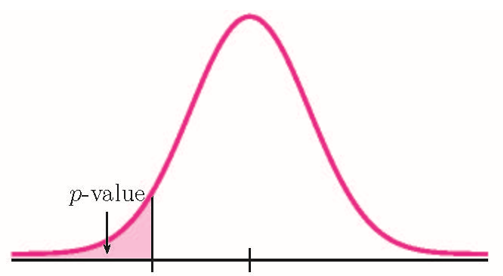
Because [latex]n_1 \times \hat{p}_1 \geq 5[/latex], [latex]n_1\times(1-\hat{p}_1)\geq 5[/latex], [latex]n_2 \times \hat{p}_2 \geq 5[/latex], and [latex]n_2\times(1-\hat{p}_2)\geq 5[/latex], the normal distribution applies, and so we use a normal distribution to calculate the [latex]p-\text{value}[/latex]. Because the alternative hypothesis is a [latex]\lt[/latex], the [latex]p-\text{value}[/latex] is the area in the left tail of the distribution.

The pooled sample proportion is:

[latex]\begin{eqnarray*}\overline{p}&=&\frac{x_1+x_2}{n_1+n_2}\\&=&\frac{6+16}{100+150}\\&=&\frac{22}{250}\\&=&0.088\end{eqnarray*}[/latex]

Function

norm.dist

Field 1

0.06-0.1066…

Field 2

0

Field 3

sqrt(0.088*(1-0.088)*(1/100+1/150))

Field 4

true

Answer

0.1010

So the [latex]p-\text{value}=0.1010[/latex].

Conclusion:

Because [latex]p-\text{value}=0.1010\gt 0.05=\alpha[/latex], we do not reject the null hypothesis. At the [latex]5\%[/latex] significance level, there is not enough evidence to suggest that the proportion of Valve As that fail under 4500 psi less than the proportion of Valve Bs that fail under 4500 psi.

NOTES

The null hypothesis [latex]p_1-p_2=0[/latex] is the claim that the proportion of valves that fail under 4500 psi is the same for both valves ([latex]p_1=p_2[/latex]). That is, the two populations have the same proportion.
The alternative hypothesis [latex]p_1-p_2\lt 0[/latex] is the claim that the proportion of Valve A’s that fail under 4500 psi less than the proportion of Valve B’s that fail under 4500 psi ([latex]p_1\lt p_2[/latex]).
Make sure to keep all of the decimal places throughout the calculation to avoid any round-off error in the [latex]p-\text{value}[/latex]. Perform the calculations of the sample proportions and the pooled sample proportion [latex]\overline{p}[/latex] in Excel and then click on the corresponding cells when completing the fields in the norm.dist function.
The [latex]p-\text{value}[/latex] of [latex]0.1010[/latex] is a large probability compared to the significance level, and so is likely to happen assuming that the null hypothesis is true. This suggests that the assumption that the null hypothesis is true is most likely correct, and so the conclusion of the test is to not reject the null hypothesis. In other words, the proportion of Valve A’s that fail under 4500 psi equals the proportion of Valve B’s that fail under 4500 psi. For the company, this means that they could not claim that the proportion of their valves that fail under 4500 psi is the smallest of all the other valves on the market.

Video: “Excel 2013 Statistical Analysis #71: Inference About Difference Between 2 Pop. Proportions Z Method” by excelisfun [28:04] is licensed under the Standard YouTube License.Transcript and closed captions available on YouTube.

Exercises

A forestry researcher wants to compare the proportion of conifers in two different parts of the country. In a random sample of [latex]100[/latex] forests in the western part of the country, [latex]56[/latex] were coniferous or contained conifers. In a random sample of [latex]80[/latex] forests in the east part of the country, [latex]40[/latex] were coniferous or contained conifers. At the [latex]5\%[/latex] significance level, is the proportion of conifers in the west part of the country greater than the proportion of conifers in the east part of the country?
Click to see Answer

Let the western part of the country be population 1 and the eastern part of the country be population 2.
- Hypotheses: [latex]\begin{eqnarray*}H_0:&&p_1-p_2=0\\H_a:&&p_1-p_2\gt 0\end{eqnarray*}[/latex]
- [latex]p-\text{value}=0.2113[/latex]
- Conclusion: At the [latex]5\%[/latex] significance level, there is enough evidence to conclude that the proportion of conifers in the west part of the country is not greater than the proportion of conifers in the east part of the country.
Two types of phone operating system are being tested to determine if there is a difference in the proportions of system failures (crashes). In a sample of [latex]150[/latex] phones with [latex]OS_1[/latex], [latex]16[/latex] had system failures within the first eight hours of operation. In a sample of [latex]150[/latex] phones with [latex]OS_2[/latex], [latex]8[/latex] had system failures within the first eight hours of operation. At the [latex]5\%[/latex] significance level, is there a difference in the proportion of system failures for the two operating systems?
Click to see Answer

Let [latex]OS_1[/latex] be population 1 and [latex]OS_2[/latex] be population 2.
- Hypotheses: [latex]\begin{eqnarray*}H_0:&&p_1-p_2=0\\H_a:&&p_1-p_2\neq 0\end{eqnarray*}[/latex]
- [latex]p-\text{value}=0.0887[/latex]
- Conclusion: At the [latex]5\%[/latex] significance level, there is enough evidence to conclude that there is no difference in the proportion of system failures for the two operating systems.
A local school district wants to compare the proportion of local high school seniors who used drugs or alcohol within the past month to the proportion of high school seniors nationwide. In a sample of [latex]100[/latex] national high school seniors, [latex]55[/latex] reported using drugs or alcohol within the past month. In a sample of [latex]100[/latex] local high school seniors, [latex]67[/latex] reported using drugs or alcohol within the past month. At the [latex]5\%[/latex] significance level, is the proportion of nationwide high school seniors who used drugs or alcohol in the past month lower than the proportion of local high school seniors?
Click to see Answer

Let the nationwide seniors be population 1, and the local seniors be population 2.
- Hypotheses: [latex]\begin{eqnarray*}H_0:&&p_1-p_2=0\\H_a:&&p_1-p_2\lt 0\end{eqnarray*}[/latex]
- [latex]p-\text{value}=0.0410[/latex]
- Conclusion: At the [latex]5\%[/latex] significance level, there is enough evidence to conclude that the proportion of nationwide high school seniors who used drugs or alcohol in the past month is lower than the proportion of local high school seniors.
Neuroinvasive West Nile virus is a severe form of the West Nile virus that affects a person’s nervous system. It is spread by the Culex species of mosquito. Last year, there were [latex]629[/latex] reported cases of neuroinvasive West Nile virus out of a total of [latex]1,021[/latex] reported West Nile cases. This year, there were [latex]486[/latex] neuroinvasive reported cases out of a total of [latex]712[/latex] reported West Nile cases. At the [latex]1\%[/latex] significance level, is the proportion of neuroinvasive West Nile cases greater this year than last year?
Click to see Answer

Let last year be population 1 and this year be population 2.
- Hypotheses: [latex]\begin{eqnarray*}H_0:&&p_1-p_2=0\\H_a:&&p_1-p_2\lt 0\end{eqnarray*}[/latex]
- [latex]p-\text{value}=0.0022[/latex]
- Conclusion: At the [latex]1\%[/latex] significance level, there is enough evidence to conclude that the proportion of neuroinvasive West Nile cases this year is greater than last year.
A researcher wants to study obesity in adults aged 18 years old and older. Adults are considered obese if their body mass index (BMI) is at least [latex]30[/latex]. In a sample of [latex]248,775[/latex] women, [latex]67,169[/latex] were considered obese. In a sample of [latex]155,525[/latex] men, [latex]42,769[/latex] were considered obese. At the [latex]1\%[/latex] significance level, is the proportion of men who are obese greater than the proportion of women who are obese?
Click to see Answer

Let men be population 1 and women be population 2.
- Hypotheses: [latex]\begin{eqnarray*}H_0:&&p_1-p_2=0\\H_a:&&p_1-p_2\gt 0\end{eqnarray*}[/latex]
- [latex]p-\text{value}=0.0003[/latex]
- Conclusion: At the [latex]1\%[/latex] significance level, there is enough evidence to conclude that the proportion of men who are obese is greater than the proportion of women who are obese.
Two computer users were discussing tablet computers. One user claims that the proportion of people under 30 years old who use a tablet is the same as the proportion of people who are 30 years old or older. In a sample of [latex]628[/latex] people under the age of 30 years, [latex]603[/latex] said they use a tablet. In a sample of [latex]2,309[/latex] people aged 30 years or older, [latex]2,251[/latex] said they use a tablet. At the [latex]1\%[/latex] significance level, is the proportion of people under the age of 30 years who use a tablet different from the proportion of people aged 30 years or older who use a tablet?
Click to see Answer

Let under 30 years be population 1 and 30 years or older be population 2.
- Hypotheses: [latex]\begin{eqnarray*}H_0:&&p_1-p_2=0\\H_a:&&p_1-p_2\neq 0\end{eqnarray*}[/latex]
- [latex]p-\text{value}=0.0489[/latex]
- Conclusion: At the [latex]1\%[/latex] significance level, there is enough evidence to conclude that there is no difference in the proportion of people in the two age groups who own a tablet.
A group of friends debated whether more men use smartphones than women. They consulted a research study of smartphone use among adults. The results of the survey indicate that of the [latex]973[/latex] men randomly sampled, [latex]905[/latex] use smartphones. For women, [latex]1,115[/latex] of the [latex]1,304[/latex] who were randomly sampled use smartphones.
1. Construct a [latex]93\%[/latex] confidence interval for the difference in the proportion of men and women who use smartphones.
2. Interpret the confidence interval in part (a).
3. Is it reasonable to claim that the proportion of men who use smartphones is higher than the proportion of women? Explain.
Click to see Answer

Let men be population 1 and women be population 2.
1. [latex]\text{Lower Limit}=0.0226[/latex] [latex]\text{Upper Limit}=0.0662[/latex]
2. There is a [latex]93\%[/latex] probability that the difference in the proportions of men and women who use smartphones is between [latex]2.26\%[/latex] and [latex]6.62\%[/latex].
3. Yes. Because both limits are positive, it suggests that the difference in the proportions is positive. That is [latex]p_1-p_2\gt 0[/latex] or [latex]p_1\gt p_2[/latex]. So the proportion of men who use smartphones is higher than the proportion of women.
Joan Nguyen recently claimed that the proportion of college-age males with at least one pierced ear is less than the proportion of college-age females. She conducted a survey in her classes. Out of [latex]107[/latex] males, [latex]20[/latex] had at least one pierced ear. Out of [latex]92[/latex] females, [latex]47[/latex] had at least one pierced ear.
1. Construct a [latex]98\%[/latex] confidence interval for the difference in the proportion of college-age males and females with at least one pierced ear.
2. Interpret the confidence interval in part (a).
3. Is it reasonable to claim that the proportion of college-age males with at least one pierced ear is less than the proportion of college-age females? Explain.
Click to see Answer

Let males be population 1 and females be population 2.
1. [latex]\text{Lower Limit}=-0.4736[/latex] [latex]\text{Upper Limit}=-0.1743[/latex]
2. There is a [latex]98\%[/latex] probability that the difference in the proportions of males and females with at least one pierced ear is between [latex]-47.36\%[/latex] and [latex]-17.43\%[/latex].
3. No. Because both limits are negative, it suggests that the difference in the proportions is negative. That is [latex]p_1-p_2\lt 0[/latex] or [latex]p_1\lt p_2[/latex]. So, the proportion of males with at least one pierced ear is less than the proportion of females with at least one pierced ear.
A business professor wants to compare the proportion of business students who work at the same time they attend school with the proportion of non-business students who work at the same time they attend school. In a sample of [latex]160[/latex] business students, [latex]110[/latex] said they work while attending school. In a sample of [latex]160[/latex] non-business students, [latex]115[/latex] said they work while attending school.
1. Construct a [latex]95\%[/latex] confidence interval for the difference in the proportion of business students and non-business students who work while attending school.
2. Interpret the confidence interval in part (a).
3. Can the professor claim that the proportions of business and non-business students who work while attending school are different? Explain.
Click to see Answer

Let business students be population 1 and non-business students be population 2.
1. [latex]\text{Lower Limit}=-0.1313[/latex] [latex]\text{Upper Limit}=0.688[/latex]
2. There is a [latex]95\%[/latex] probability that the difference in the proportions of business students and non-business students who work while attending school is between [latex]-13.13\%[/latex] and [latex]6.88\%[/latex].
3. No. Because [latex]0[/latex] is inside the confidence interval, it suggests that the difference in the proportions is [latex]0[/latex]. That is [latex]p_1-p_2=0[/latex] or [latex]p_1=p_2[/latex]. S,o the proportion of business students who work while attending school is the same as the proportion of non-business students.

“9.5 Statistical Inference for Two Population Proportions” and “9.6 Exercises” from Introduction to Statistics by Valerie Watts is licensed under a Creative Commons Attribution-NonCommercial-ShareAlike 4.0 International License, except where otherwise noted.

License

Icon for the Creative Commons Attribution-NonCommercial-ShareAlike 4.0 International License

Introduction to Statistics - Second Edition Copyright © 2025 by Valerie Watts is licensed under a Creative Commons Attribution-NonCommercial-ShareAlike 4.0 International License, except where otherwise noted.

Constructing a Confidence Interval for the Difference in Two Population Proportions

NOTES

NOTE

NOTES

Conducting a Hypothesis Test for the Difference in Two Population Proportions

NOTES

NOTES

NOTES

NOTES

Exercises

License

Share This Book