6.2 Supporting Domestic Production, Employment, and Well-Being

Most “second-best world” arguments for protection contend that an industry should be favoured over imports because additional social benefits can be obtained from domestic production and employment. Some variations of this basic view are the following:

• There are spillover benefits from domestic production that accrue to other industries and businesses in the economy.
• Employment in the industry generates worker competencies and attitudes that benefit other industries and businesses.
• Protection of a nascent industry with high production costs will lead to efficient, internationally competitive industries over time.
• Protection of an industry facing relentless import competition may be warranted to support the income of workers as they transition to other avenues of employment.
• It is important to support production in industries that are critical to national security.

At the heart of these arguments is the idea that social benefits are not fully captured by private production and employment, and therefore, government intervention is necessary to protect the domestic industry from import competition.

In the analysis that follows, we will examine the situation of a small country that promotes production in an industry because it generates external benefits by using an import tariff.

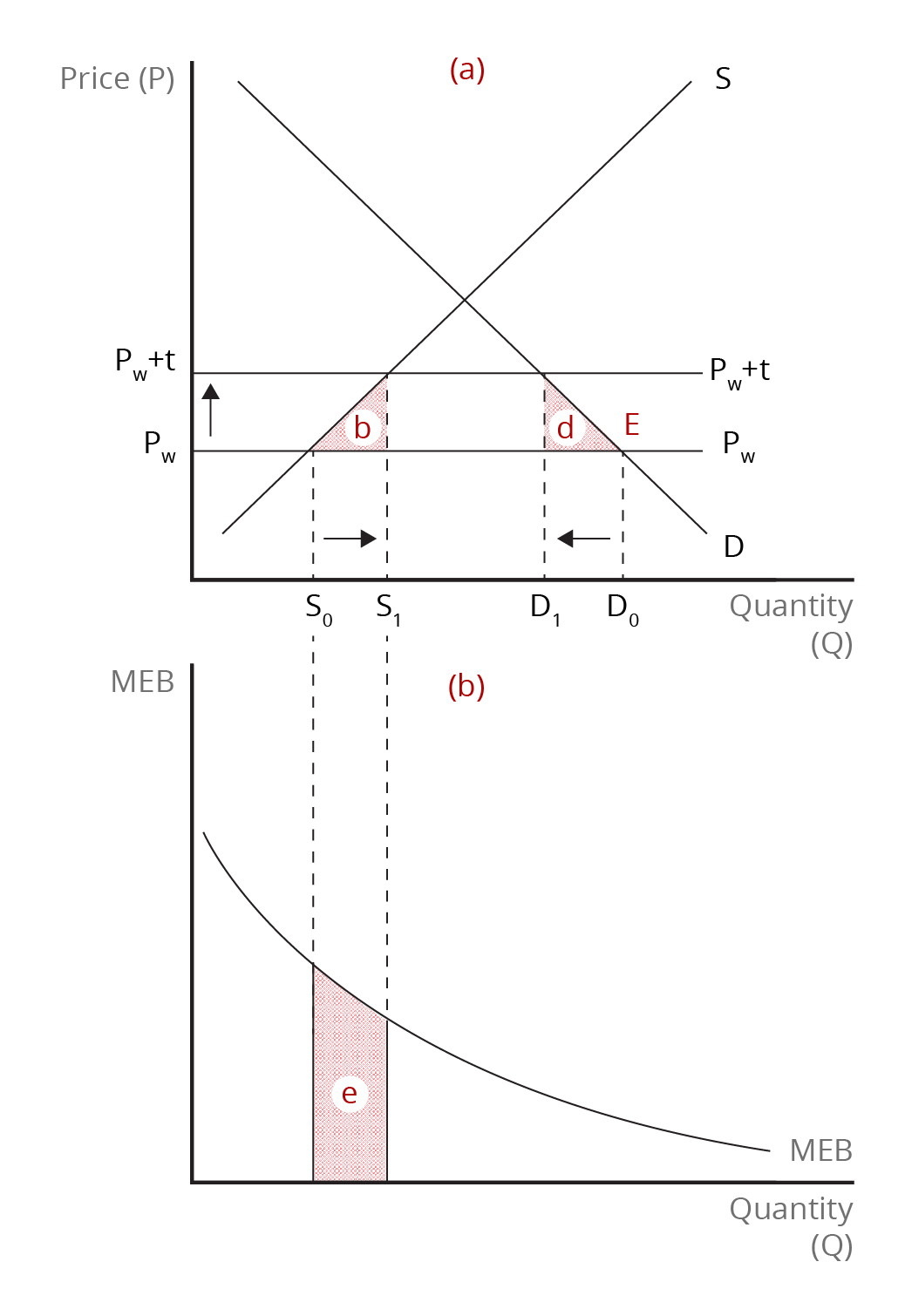
Before the small country engages in international trade, the domestic price is high, as indicated by the intersection of the domestic supply curve [latex](\text{S}_{d})[/latex] and the domestic demand curve [latex](\text{D}_{d})[/latex] in Panel (a) of Figure 6.2. In light of its inability to influence the world price, the small country can purchase any amount of the product at the prevailing world price [latex](\text{P}_{w})[/latex]. The world price is indicated by a horizontal line that lies below the domestic equilibrium. With international trade, equilibrium in the domestic market is at point [latex]\text{E}[/latex], where the quantity purchased by domestic consumers is [latex]\text{D}_{0}[/latex] and the quantity supplied is [latex]\text{S}_{0}[/latex]. The difference between [latex]\text{D}_{0}[/latex] and [latex]\text{S}_{0}[/latex] represents the level of imports before the tariff is imposed.

As we have seen earlier, the domestic price increases when the import tariff is imposed. The new domestic price is represented by the horizontal line, [latex]\text{P}_{w}+{t}[/latex], where [latex]\textit{t}[/latex] is the tariff. The higher domestic price causes domestic consumers to buy a smaller quantity, [latex]\text{D}_{1}[/latex] and domestic producers to boost their level of production to [latex]\text{S}_{1}[/latex]. As a result, the level of imports falls from [latex]\text{D}_{0}-\text{S}_{0}[/latex] to [latex]\text{D}_{1}-\text{S}_{1}[/latex]. The small country suffers the usual deadweight losses of the production effect (area [latex]\textit{b}[/latex] ) and the consumption effect (area [latex]\textit{d}[/latex] ). With the import tariff, the country is now choosing to substitute higher-cost domestic production for lower-cost imports and discouraging some purchases to which consumers attach a higher value than indicated by the world price.

However, our small country derives additional social benefits from domestic production that is not captured by domestic producers themselves. Such additional benefits may stem, for instance, from national security concerns or transferable worker skills. This situation is indicated in the Panel (b) of Figure 6.2, which shows the marginal external benefits from production. As production increases, the additional external benefit declines, which gives us a downward-sloping marginal external benefit curve (MEB). Production is measured on the same scale in both Figure 6.2 (a) and Figure 6.2 (b). The additional social benefit that results from the increase in domestic production due to the import tariff is indicated by area [latex]\textit{e}[/latex]. Whether the country eventually gains or loses economic well-being depends on whether the additional social benefits (area [latex]\textit{e}[/latex] ) exceed the deadweight losses due to the production and consumption effects (areas [latex]\textit{b}[/latex] and [latex]\textit{d}[/latex] ). If area [latex]\textit{e}[/latex] is greater than the sum of areas [latex]\textit{b}[/latex] and [latex]\textit{d}[/latex], then our small country will be better off from the tariff.

We have seen that the protection of a domestic industry with an import tariff can improve a country’s economic well-being if external benefits are present. However, supporting the industry with an import tariff may not be the appropriate “second-best” policy. We will now compare an import tariff with a production subsidy to evaluate which policy is more efficient from the standpoint of society as a whole.

Image Descriptions

Figure 6.2: Protecting Domestic Production with an Import Tariff

The image comprises two vertically arranged graphs, the top labelled (a) and the lower labelled (b). Graph (a) is a supply-and-demand graph with price (P) on the vertical axis and quantity (Q) on the horizontal axis.

There are two intersecting lines: a downward-sloping demand line (labelled D) and an upward-sloping supply line (labelled S). Two horizontal lines extending from the lower half of the y-axis are labelled P_w+t and P_W. A vertical arrow points up from P_w to P_w+t. The intersection of D and P_W is labelled “E.”

Four quantity levels are marked along the horizontal axis, S₀, S₁, D₁, and D₀, with dotted horizontal lines up to the intersections of the price lines with the supply and demand curves. A horizontal arrow points right from S₀ to S₁; another arrow points left from D₀ to D₁.

Area b is a shaded triangle formed by S, P_W and S₁. Area d mirrors b, formed by D₁, P_W, and D.

Graph (b) includes a vertical axis labelled MEB, and a horizontal axis labelled Quantity (Q). A single curved line sloping downwards from left to right, beginning from two-thirds up the y-axis to the end of the x-axis, is labelled “MEB.” Dotted lines extend down from the S₀ and S₁ marks on the x-axis of graph (a). Area e is the shaded space below the MEB line and between the dotted lines.

[back]