3.3 Alternative Theories of International Trade

The first alternative theory that we consider is based on monopolistic competition and product differentiation. This theory provides the foundation to the main explanation for intra-industry trade – two-way trade in similar products. Next, we consider a model which illustrates how substantial internal economies of scale lead to a global oligopoly. Last, we discuss a model which demonstrates how external economies of scale can lead to the formation of industry clusters in a few countries. For all of these theories, we examine their implications for the pattern of trade, the terms of trade, and the division of the gains from trade.

Monopolistic Competition, Product Differentiation, and International Trade

To gain insight into why intra-industry trade is prevalent among developed countries, we consider a model of trade based on monopolistic competition. In this industry, there are limited external economies of scale, which implies that there is room for many firms. Firms in the industry supply different versions of the same basic product so that products are differentiated. Last, firms are free to enter and exit the industry in response to economic profits. If economic profit is positive, new firms enter, and if economic losses are occurring, some firms leave the industry. Since firms supply differentiated products, they have some pricing power. In the long run, firms in the industry earn zero economic profit as above-normal profits are eliminated by competition.

The Market Without International Trade

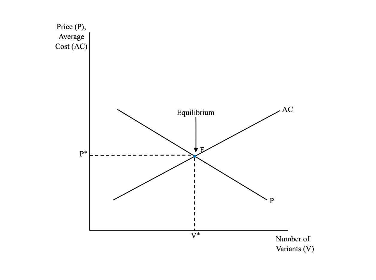
The domestic market before trade is characterized by a price curve, [latex]\text{P}[/latex], and an average cost curve, [latex]\text{AC}[/latex] (see Figure 3.2). The former represents the demand side of the market, and the average cost curve represents its supply side. The price curve relates the number of product varieties on the horizontal axis to the price of the broad product. With only a very limited number of varieties available, the product price is relatively high. However, as more and more product varieties become available on the market, the typical firm loses pricing power, as each new variety represents a substitute and, therefore, an increase in competition. Price, therefore, falls with the introduction of more and more product varieties. The price curve, therefore, is downward sloping. It is also relatively flat, indicating a considerable degree of competition in the market.

Regarding the supply side, the typical firm is not able to fully take advantage of the available internal economies of scale. As increasingly more varieties of the product are introduced, individual versions are produced in smaller and smaller volumes, given the size of the market. This reduces the ability of firms to benefit from internal economies of scale. That is, the larger the number of product versions, the smaller the level of output per version, and the more limited the opportunity for exploiting economies of scale. Average cost increases as the scale of production of individual varieties falls. The average cost curve, therefore, slopes upward – the introduction of more product versions in a given market raises the average cost.

Bringing together the demand and supply sides of the market, we can determine the equilibrium price and the equilibrium number of product varieties that result. The price and unit cost curves are shown, respectively, as [latex]\text{P}[/latex] and [latex]\text{AC}[/latex] in Figure 3.2. The equilibrium price and equilibrium number of varieties, indicated respectively as [latex]\text{P*}[/latex] and [latex]\text{V*}[/latex], are given by the intersection of the price and unit cost curves. At the point of intersection, price is equal to average total cost, and firms in the industry are earning zero economic profit in long-run equilibrium. This represents the situation prior to trade, as depicted in Figure 3.2.

Allowing for International Trade

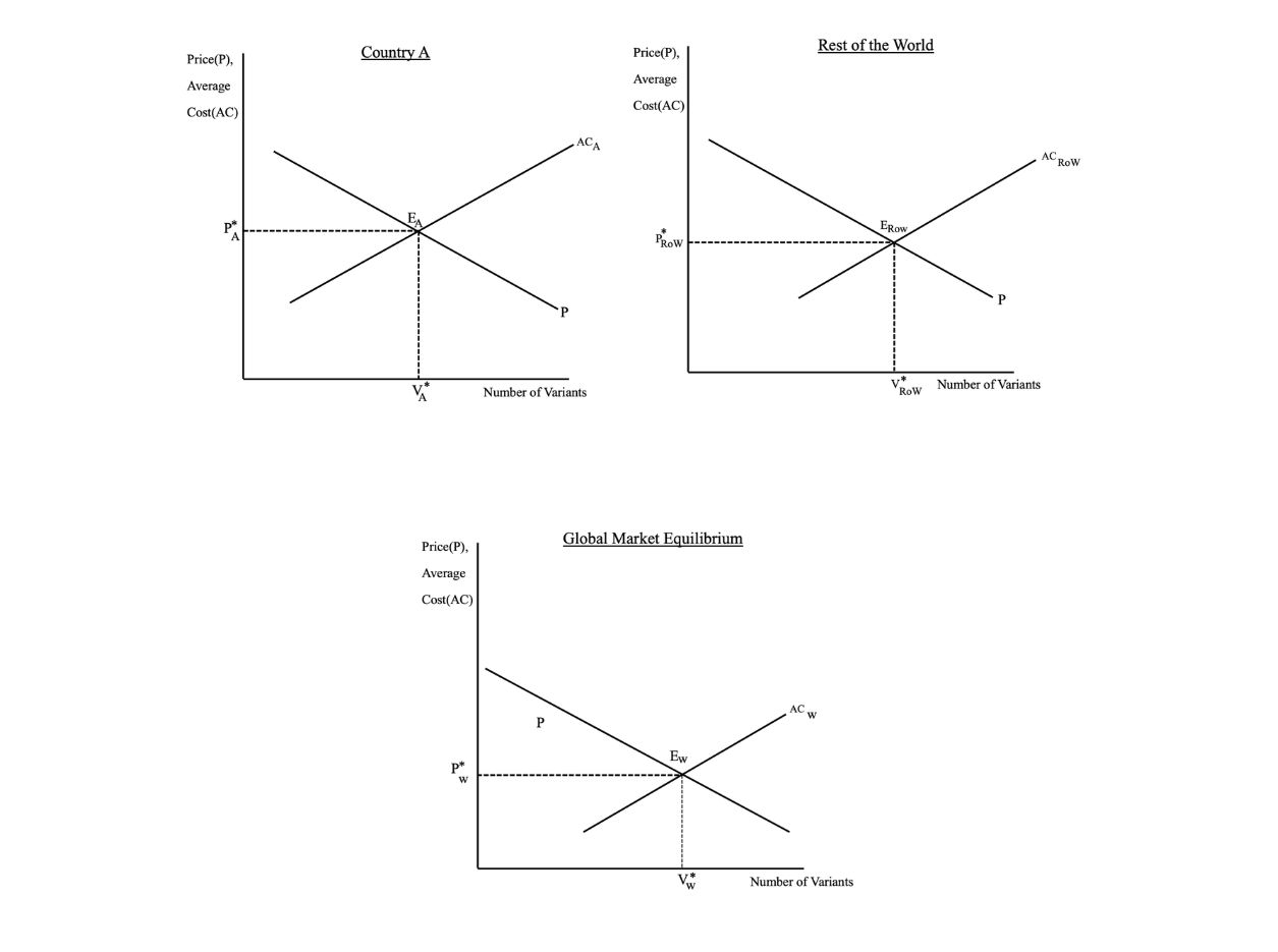
To allow for international trade, we presume that equilibrium initially exists in monopolistically competitive markets for the same product in two different countries, Country A and the Rest of the World (RoW). We assume that the market in the rest of the world is larger than the market of Country A, which allows for greater economies of scale to be attained. This means that the average cost curve [latex]\text{(AC)}[/latex] lies further to the right than the [latex]\text{AC}[/latex] curve for the domestic market in Country A (see Figure 3.3). Given similar demand conditions in both countries, the demand curve is the same for the RoW as it is for Country A. Given the larger market in the RoW and the achievement of greater economies of scale, the equilibrium price of the typical variety in the RoW is lower and the equilibrium number of varieties is larger.

With the opening up of trade, the two domestic markets become one integrated market, the world market. The bigger market allows firms to produce larger quantities and locate at lower points along their long-run average cost curves—that is, firms are better able to exploit economies of scale. This means that the aggregate average cost curve lies further to the right than either the Country A curve or the RoW curve. The world price curve is the same as those for the national markets prior to trade on the assumption that demand conditions are similar across trading countries. The resulting equilibrium price for the typical variety is lower and the equilibrium number of varieties is larger in the world market. With greater exploitation of scale economies and more competition, price falls, and a larger number of varieties is offered for sale to consumers. This situation is depicted in Figure 3.3.

With the opening up of trade, firms from Country A can export their versions of the product to the rest of the world because foreign buyers have a preference for Country A’s products. Similarly, firms from the RoW can export their varieties to Country A because some buyers in Country A prefer products from the rest of the world.

Figure 3.3 shows the equilibrium in the domestic markets for Country A and the Rest of the World before international trade and equilibrium in the global market with trade.

The Basis for Trade

Economies of scale do not provide any particular production cost advantage to firms in any specific country since we assume that technology is the same across countries. Thus, economies of scale do not form the basis of trade in this model. Instead, a country’s engagement in international trade is driven by product differentiation; that is, a country exports when domestic production of unique versions of the product is demanded by some consumers in foreign markets and imports when some consumers in this country demand particular varieties of the same basic product made by firms in other countries. Therefore, intra-industry trade in differentiated products can be significant, even between countries that are similar in their resource endowments and technologies.

Gains from Trade

Monopolistic competition, product differentiation, and intra-industry trade provide additional important insights into national gains from trade and the effects of trade on the well-being of different groups within a country. In this model, an additional source of national benefit from trade comes from the broader product range that is now available to consumers as a result of imports. In addition, with intra-industry trade, there is little or no effect on the distribution of factor incomes – evident in the H-O model – as inter-industry shifts in production and resource use are limited. This is because exports offset any domestic market share losses that may arise from imports. To the extent that any losses in factor incomes arise due to inter-industry production shifts, these losses will likely be compensated for by the gains to consumers from greater product diversity.

Global Oligopoly and International Trade

An industry in which a few firms in different countries account for the bulk of the world’s production is a global oligopoly. In a global oligopoly, firms benefit from substantial internal economies of scale, which allows only a small number of plants located in a few countries to populate the global industry. These large firms choose plant locations to maximize profits, and inherent advantages stemming from production and demand conditions are likely to be important considerations in this decision. The presence of substantial economies of scale has implications for the pattern of international trade, the pricing strategies of firms within the global oligopoly, and the division of the welfare gains from trade both within and between countries.

Countries that have the production facilities of the global oligopoly become the exporters of the product, while other countries become the importers. Firms in an oligopoly, because they are few, usually recognize their interdependence, and this influences their pricing strategy. Oligopolistic firms may choose to collude and set high prices or to compete aggressively, which leads to low prices. If firms pursue the former pricing strategy, they can earn above-normal economic profit. If firms adopt the latter strategy, any positive economic profit is eroded by competition – firms earn only a normal return. In general, it is not possible to say which price and output strategy the firms will adopt, and therefore, we present the two extremes of collusion and competition.

Pricing is critical for the distribution of gains from trade. If oligopolistic firms compete on price, output would be larger with a low price. Thus, more of the gains would go to foreign buyers and the importing country and less to the firms themselves. If firms in the industry jointly restrict output, they would earn significant economic profit on export sales and earn higher export prices. The better terms of trade mean that the firms and exporting countries gain surplus at the expense of consumers in importing countries. Moreover, the small number of countries that produce the industry’s output can sustain these gains over time. To the extent that the oligopolistic firms benefit from substantial scale economies, they would be able to fend off competition from potential entrants.

External Economies of Scale, Clustering, and International Trade

Let us now turn our attention to an industry benefiting from substantial external economies of scale. External economies of scale arise when the expansion of an industry in a particular geographic area causes long-run average costs to fall for all firms in the industry in the area. To see the effects of external economies of scale, we consider a competitive industry with a large number of firms in each location and no internal economies of scale. This means that in the industry, there are many small firms which have no influence over price and obtain zero economic profit in the long run. However, the industry benefits from external economies of scale – as it expands, the average cost of the typical firm declines.

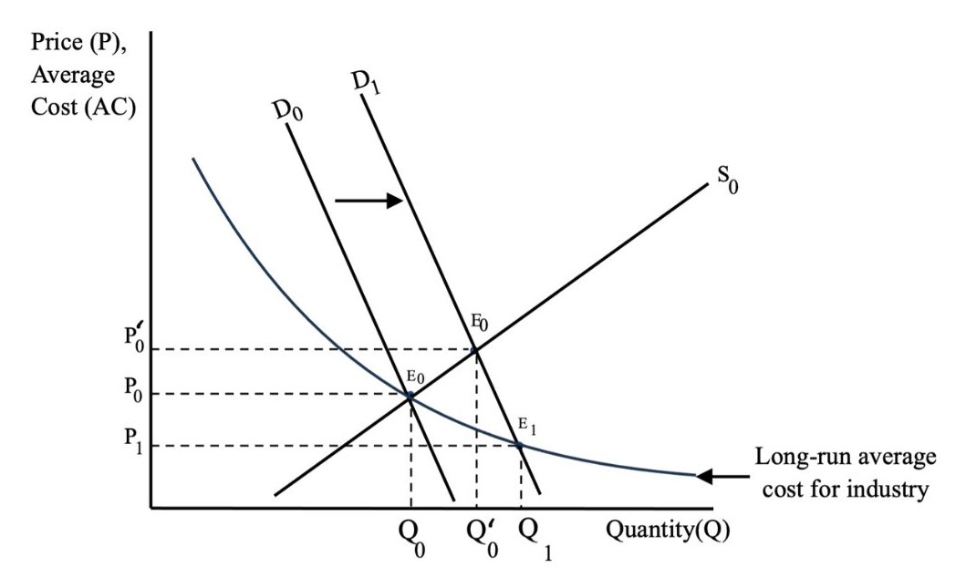
To analyze the implications of an industry benefiting from large external economies of scale, let us establish the initial position of the industry prior to an event which causes it to expand. The industry is in long-run equilibrium, with equilibrium output and price determined by the interaction of industry demand and supply. Graphically, the industry supply and demand curves intersect each other along the industry’s downward-sloping long-run average cost curve (see Figure 3.4). This indicates that, in long-run equilibrium, price is equal to average cost, which means that firms are making zero economic profit.

Now, suppose a shift in the preferences of foreign consumers brings about an increase in industry demand and lifts exports. Graphically,  the demand curve shifts rightward and causes both price and industry output to increase in the short term. The larger production level facilitates the achievement of further external economies of scale, and average costs fall throughout the national industry. This causes the industry supply curve to shift outward to the right, and eventually, a new equilibrium is achieved at the point of intersection of the new supply and new demand curves. At this point, the industry is situated further down the industry’s long-run average cost curve, resulting in a larger output, lower average cost, and a lower price. This situation is depicted in Figure 3.4.

In terms of economic well-being, producers in the exporting country gain economic surplus with the expansion of industry output. Producers in the importing country lose surplus in the face of increased import competition. Consumers in the importing country gain economic well-being considering the lower price and the increased consumption. Consumers in the exporting country also benefit from the fall in price and expanded consumption. This last result contrasts with the standard case of comparative advantage models in which the reduced domestic availability of the product due to exports causes the price in the exporting country to rise. Here, consumers in the exporting country experience an increase in surplus, whereas in the standard case, they would experience losses.

With external economies of scale, if international trade opens up, production tends to become concentrated in a few locations. Clusters of firms in some locations will expand production, and countries with those locations will export the product. Other countries will import the product as their production levels shrink. Once production is established, new potential locations cannot easily overcome the scale advantages of the established locations. As a result, dynamic gains accrue to firms that initially become established.

Image Descriptions

Figure 3.2: The Domestic Market Before Trade: Equilibrium

The image displays a graph with a vertical axis labelled “Price (P), Average Cost (AC)” and a horizontal axis labelled “Number of Variants (V).” A downward-sloping line labelled “P” intersects an upward-sloping line labelled “AC” at a point labelled “E.” There is an arrow labelled “Equilibrium” pointing down to point E. Dashed horizontal and vertical lines extend from the equilibrium point to the respective axes, intersecting at “P*” on the vertical axis and “V*” on the horizontal axis.

[back]

Figure 3.3: Equilibrium in the Global Market

The image contains three separate graph. The first graph is labelled “Country A,” and is side-by-side with the second, labelled “Rest of the World.” The centred beneath these two is the third graph, labelled “Global Market Equilibrium.” Each graph features a standard supply and demand graph layout with two axes. The vertical axis is labelled “Price (P) Average Cost (AC),” while the horizontal axis is labelled “Number of Variants.” The graphs display two intersecting lines: a downward-sloping line representing average cost and an upward-sloping line representing price. The intersection of these lines is labelled E. There is a dotted horizontal line from E to the vertical axis labelled P* and a dotted vertical line from E to the horizontal axis labelled V*. Each graph’s points and labelled are distinguished with subscript A for Country A, ROW for Rest of World, and W for Global Market. The dotted lines in the Country A graph form a square that is a quarter of the graph. The dotted lines in the Rest of the World graph form a rectangle that is a little shorter and much longer than the Country A square. The dotted lines in Global Market Equilibrium are much shorter than the rectangles in the Rest of the World.

[back]

Figure 3.4: The Impact of External Economies of Scale in a Competitive Industry

The image is a graph with “Price (P), Average Cost (AC)” on the vertical y-axis and “Quantity (Q)” on the horizontal x-axis. There are two demand curves labelled D₀ and D₁, which intersect with a supply curve S₀. An arrow shows the shift right from D₀ and D₁. A downward-sloping concave curve originating to the left of D₀ is labelled “Long-run average cost for the industry.”

The Long-run average cost line intersects D₀ and S₀ at point E₀, and D₁ at E₀ prime. D₁ and S₀ also intersect each other at E₁.

Three horizontal dashed lines extending from the E intersections to the y-axis are labelled from the top, P₀ prime, P₀ and P₁. Three vertical dashed lines extending from the E intersections to the x-axis are labelled from the left Q₀, Q₀ prime and Q₁.

[back]