2.4 Production and Consumption, Before and After Trade

To determine the best combination of consumption quantities of two goods for a nation, we must bring together the supply and demand sides of the economy. That is, we must bring together the production possibilities frontier (PPF) and the map of community indifference curves. To determine the benefits of international trade, we compare the best combination of production and consumption quantities for the nation before and after international trade.

Before International Trade

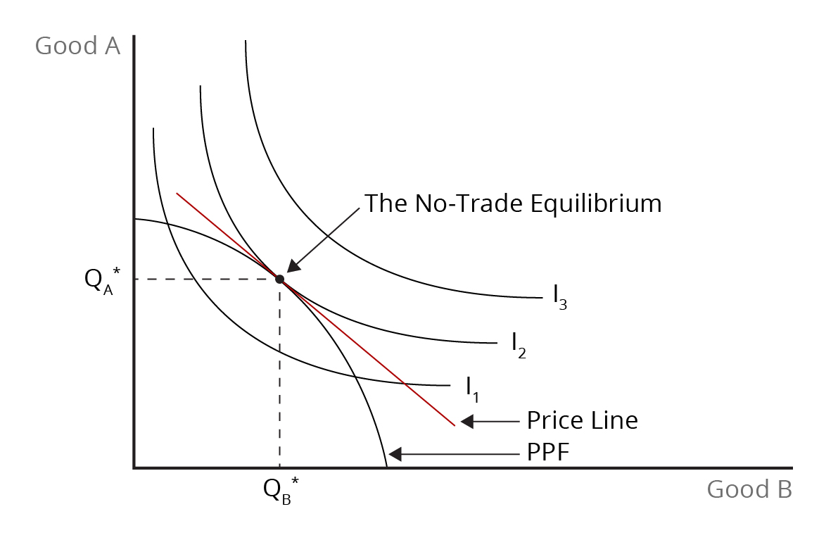
Before trade, a country must produce the combination of quantities of the two products that maximizes the nation’s economic well-being. That is, a country must allocate its resources so that it achieves the maximum benefit at the lowest cost of resources. The relative resource cost – i.e., the opportunity cost of production – is given by the slope of the PPF. Meanwhile, the relative price that society is willing to pay is given by the slope of a community indifference curve. The nation will choose the combination of the quantities of the two products so that the marginal opportunity cost (i.e., the cost ratio) is equal to the relative price (i.e., the price ratio). At that point, the value of national production is maximized before trade.

Graphically, this means that the nation chooses a combination of production and consumption quantities indicated by the point of tangency between the nation’s PPF and the highest attainable community indifference curve. At that point, the value of national production is maximized in the absence of trade – that is, the nation will have allocated its resources to get the highest benefit at least cost. At the no-trade equilibrium, the quantities of the two goods produced are the same as the consumption quantities.  Figure 2.8 shows the no-trade equilibrium for the nation, i.e., the best quantity combination of the two goods.

After International Trade

To introduce international trade, we must consider the equilibria before trade in two different countries. Since the PPFs and marginal opportunity costs will be different for both countries, relative prices will differ. The difference in relative prices before trade provides the immediate reason for trade. The country that produces a good at a lower opportunity cost will export it and import the other good. The price of the export good will rise in both countries due to the additional source of demand. Meanwhile, the price of the import good will fall due to increased availability in the domestic market. In both countries, producers will respond to the higher price of the export good by producing more and to the lower price of the import good by producing less.

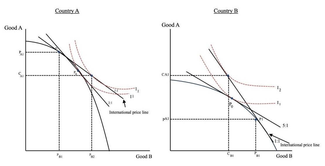
Because both countries are now producing more of the export good, they can now sell excess production of the good in which they have a comparative advantage and use the earnings to satisfy the deficits that emerge for the good in which they are at a comparative disadvantage. The respective points of consumption for both countries will lie along the international price line (i.e., the international terms of trade line), which is tangent to the respective PPFs at the after-trade points of production. Both countries will trade along the international price line away from their after-trade points of production until each reaches a point of tangency with the highest attainable community indifference curve.

Once we have established the production and consumption quantities for the two countries after trade, we can determine the quantities of imports and exports. Exports arise if production is larger than domestic consumption, while imports result if production is less than consumption. We find that, in equilibrium, trade is balanced for both products, with exports from one country being equal to imports into the other. We can summarize the export and import quantities for both countries using trade triangles, which are bounded by export and import quantities and the international price line. Figure 2.9 shows the free trade equilibrium and the effects of free trade on production, consumption, and international prices.

The Benefits from Trade

International trade provides benefits for the participating countries. We can demonstrate the gains from international trade in two ways. The first is that trade allows each country to consume a combination of the quantities of the two goods that lie beyond its PPF. We presume that a nation would prefer more consumption to less. Second, international trade allows each country to reach a higher community indifference curve than it would otherwise. However, we must recall that using community indifference curves to show national gains may hide the fact that trade may benefit some groups while hurting others.

The extent to which each country benefits from international trade depends on the international terms of trade. The international terms of trade are equal to the export price divided by the import price. The better the terms of trade for a particular country, the greater the gains from international trade as the country will be able to attain a higher community indifference curve. Stated differently, a higher export price (along with greater production) means higher income, which facilitates higher national consumption and economic well-being.

Trade Affects Production and Consumption

International trade affects the levels of domestic production and consumption of the two goods. There are two types of impacts on production. First, within each country, production expands for the export good and falls for the import good, as the expanding industry bids resources away from the shrinking import industry. With increasing marginal opportunity costs, each country only partially specializes in the production of the export good. Second, the shift from the situation before trade to the situation after free trade results in more efficient global production. This is because each country increases the production of the good in which it is initially the lower-cost producer. Efficiency gains result in increased global production with international trade compared with the situation before trade.

In each country, trade also alters the consumption quantities for each product. Based on the substitution effect, the population of each county purchases more of the imported product whose price has fallen because of international trade. In addition, the increase in real income in both countries as average prices fall allows consumers to purchase more of the imported product. Thus, consumption of the imported good definitely increases. However, the consumption quantities of the exported product may increase, decrease, or remain the same after trade, depending on whether the negative substitution effect is smaller than, larger than, or equal to the positive income effect. Overall, though, consumption in both countries will increase.

What Determines the Pattern of Trade

The immediate basis for international trade is that relative prices for particular products differ between countries before trade. But why do prices differ? Prices may differ because the production conditions between countries differ due to resource availability or the state of technology. Prices can also vary because of differences in domestic demand conditions and differences in economies of scale. Economies of scale lower average production costs and, therefore, can reduce prices. Another factor that can cause prices to differ between countries before trade is differences in government policies. Some policies, such as input taxes and regulation, can raise prices, while other policies (e.g., input subsidies) can lower prices. Conventional theories of international trade assume that demand conditions are similar and focus on production conditions as the reason for initial price differences across countries.

Image Descriptions

Figure 2.8: Bringing Production Possibilities and National Preferences Together

A graph with the vertical axis labelled “Good A” and the horizontal axis labelled “Good B.” A concave curve labelled as “PPF” (Production Possibility Frontier) slopes downward from the middle upper left to the middle-lower right. A straight line labelled the “Price Line” runs as a tangent on PPF. Three convex indifference curves are labelled I₁, I₂, and I₃. The point where the price line is tangent to the PPF and I₂ is labelled “The No-Trade Equilibrium” and is marked by a dot with a vertical and a horizontal dashed line extending to the axes to indicate the equilibrium quantities of Good A (Q_A) and Good B (Q_B).

[back]

Figure 2.9: The Effects of Free Trade on Production, Consumption, and Price

The image contains two graphs titled Country A on the left and Country B on the right. Each graph has two axes: the vertical axis is labelled “Good A” and the horizontal axis is “Good B.” The points where the axes intersect are in the lower left corner.

Country A has a downward convex curve, and two downward sloping lines, which are labelled 2:1 and 1:1, all intersect each other towards the top of the graph; the 1:1 line extends further along the x-axis and is labelled “International price line.” To the right of and tangent to each sloping line is a dotted concave curve, labelled l₁ and I₂, respectively. The intersection of the sloping lines and dotted curves is marked by dots. The dot on the upper left of the graph, which is on the convex curve and International price line, is labelled P₁. To the right and down, a dot marks the intersection of the convex curve, the 2:1 line and I₁ and is labelled P₀. Slightly down and to the right, the dot on the International Price line and I₂ is not labelled. P₁ has a horizontal dotted line to the axis marked P_A1 and a vertical dotted line to the axis marked P_B1. The unlabelled dot has a horizontal dotted line to the axis marked C_A1 and a vertical dotted line to the axis marked P_B2.

Country B is similar to Country A, but the lines and curves have different positions. The downward convex curve begins lower on the vertical axis and ends further out on the horizontal axis.  The International price line slopes more steeply and is labelled 1:1. The second line is labelled 5:1 and begins lower on the vertical axis and extends further on the horizontal axis than the International price line. An unlabelled dot in the center marks the intersection of the International price line and I₂, with a horizontal dotted line to the axis marked C_A1 and a vertical dotted line to the axis marked C_B1. Below this is dot P₀, which is the intersection of the convex curve, the 5:1 line, and I₁ curve. To the right and further down is dot P₁, where the International price line and the convex curve meet; the horizontal dotted line from this dot to the axis is labelled P_A1 and the vertical dotted line to the axis is labelled P_B1.

[back]