6.3 Comparing an Import Tariff with a Production Subsidy

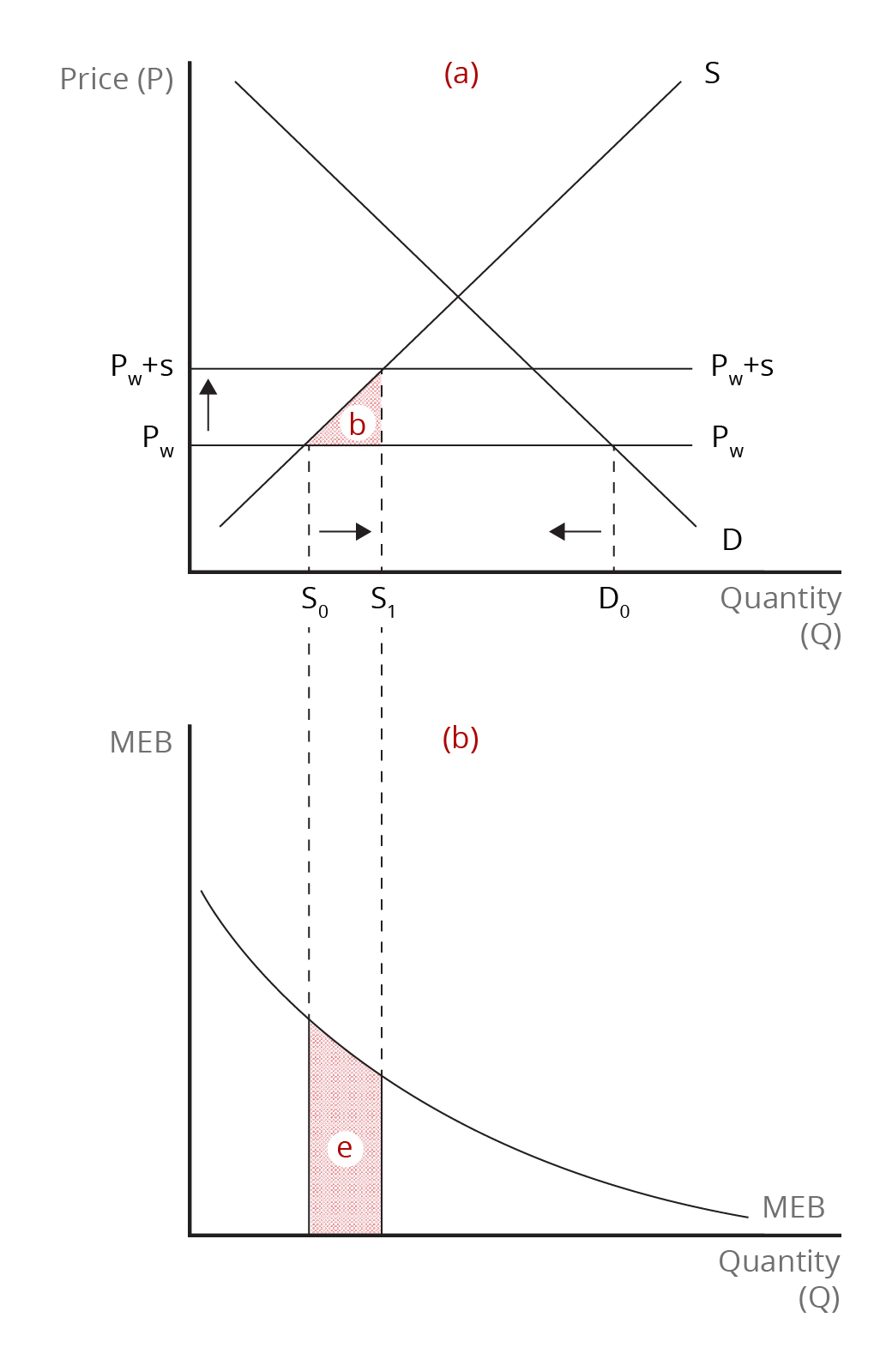
An alternative to an import tariff to support the domestic industry is the use of a production subsidy. As in the case of an import tariff, a production subsidy increases the domestic price over the world price. However, it does so only for domestic producers. In Figure 6.3, presuming the small country is involved in international trade, the domestic price is equal to the world price, [latex]\text{P}_{w}[/latex] before the production subsidy is granted. With the production subsidy, the price that domestic producers receive increases to [latex]\text{P}_{w}+\textit{s}[/latex], where [latex]\textit{s}[/latex] represents the subsidy. On the assumption that the subsidy is equivalent to the import tariff, producers respond by boosting production to the same extent. As in the case of the tariff, higher-cost domestic production is substituted in consumption for lower-cost imports. With domestic production increasing from [latex]\text{S}_{0}[/latex] to [latex]\text{S}_{1}[/latex], the nation suffers the usual deadweight loss of the production effect – it loses area [latex]\textit{b}[/latex].

However, there will be no deadweight loss from the production subsidy for our small country due to the consumption effect (area [latex]\textit{d}[/latex] ). This is because the subsidy does not raise the price that consumers pay for the product. Domestic consumption does not fall as consumers continue to pay the world price Pw. Since the external benefit is the same in the case of the tariff as for the subsidy, the latter produces an outcome in terms of net national well-being that is superior. Since the external benefit occurs in production, it is better to address the distortion in a way that does not change the price consumers pay. Our small country will gain economic well-being with a production subsidy if the external benefits exceed the deadweight loss due to the subsidy; that is, if the size of area [latex]\textit{e}[/latex] exceeds the size of area [latex]\textit{b}[/latex].

Our conclusion is that the net benefit of the production subsidy is greater than that of an import tariff because the nation does not incur the consumption effect (area [latex]\textit{d}[/latex] ). However, for this to be true, we assume that no other gaps between private and social incentives emerge as a result of the government having to pay for the subsidy. In short, we must assume that additional net social losses do not arise because the government must raise additional taxes or cut spending on competing policies. Raising income taxes changes people’s incentives to earn additional income through incremental effort. In addition, if government spending reallocated to fund the subsidy had previously been providing public goods worth more than their marginal cost, there is a further social cost incurred.

Suppose that, instead of boosting production, the government’s aim was to preserve jobs in the import-competing industry. Then, the same basic conclusions will hold, namely, a production subsidy would be a superior policy to trade protection in the form of an import tariff in that it helps domestic producers without hurting consumers. However, it is possible to improve upon this policy by targeting its application even more closely to the source of the problem. If the problem lies with the number of jobs in the industry, then it would be better to link the subsidy to the number of employed workers.

Image Descriptions

Figure 6.3: Supporting Domestic Production with a Production Subsidy

The image comprises two vertically arranged graphs, the top labelled (a) and the lower labelled (b). Graph (a) is a supply-and-demand graph with price (P) on the vertical axis and quantity (Q) on the horizontal axis.

There are two intersecting lines: a downward-sloping demand line (labelled D), and an upward-sloping supply line (labelled S). Two horizontal lines extending from the lower half of the y-axis are labelled P_W+s and P_W. A vertical arrow points up from P_W to P_W+t. The intersection of D and P_W is labelled “E.”

Three quantity levels are marked along the horizontal axis, S₀, S₁, and D₀, with dotted vertical lines up to the intersections of the price lines with the supply and demand curves. A horizontal arrow points right from S₀ to S₁; another arrow points left from D₀ toward S₁.

Area b is a shaded triangle formed by S, P_W and S₁.

Graph (b) includes a vertical axis labelled MEB, and a horizontal axis labelled Quantity (Q). A single curved line sloping downwards from left to right, beginning from two-thirds up the y-axis to the end of the x-axis, is labelled “MEB.” Dotted lines extend down from the S₀ and S₁ marks on the x-axis of graph (a). Area e is the shaded space below the MEB line and between the dotted lines.

[back]