3.5 Economic Growth and Its Implications for Trade

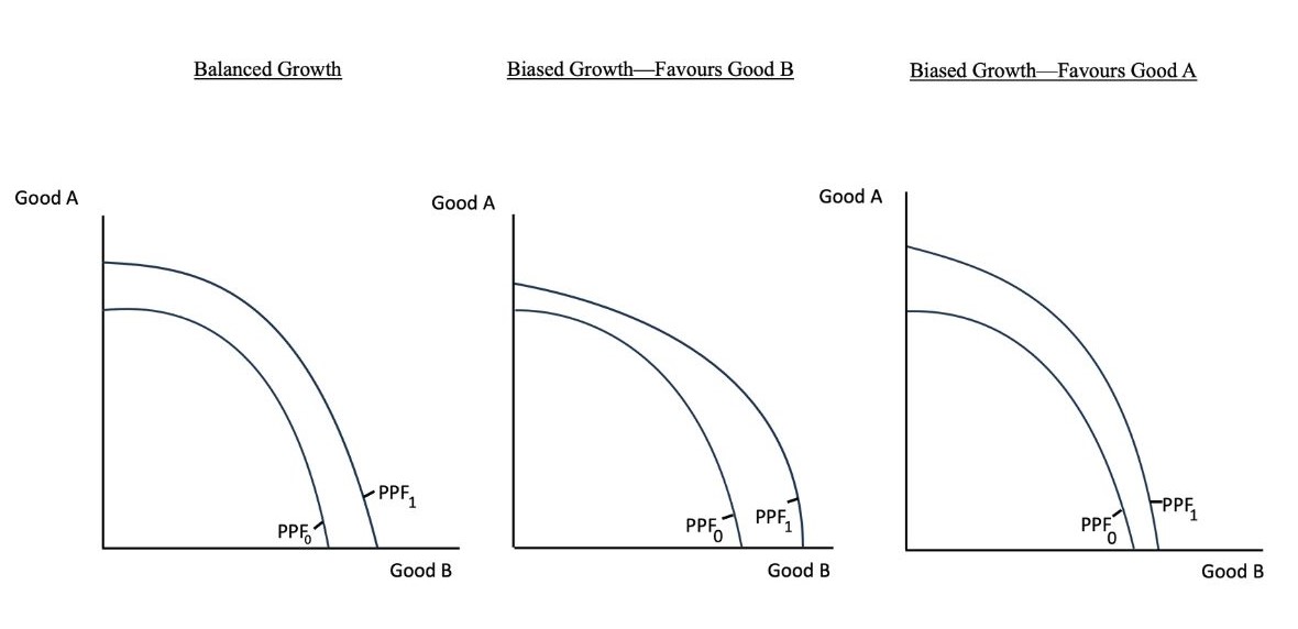
Economic growth has implications for a country’s involvement in trade (Pugel, 2020). Economic growth is due to an increase in a country’s production capabilities. There are two basic sources of economic growth, namely, increases in a country’s resource endowments and technological improvements. Graphically, an expansion of a country’s production capabilities causes an outward shift in its production possibilities frontier (PPF), as in Figure 3.5. A country can experience balanced economic growth or growth biased toward the production of particular goods.

In the case of balanced growth, the PPF shifts outward proportionately. This would result in an increase in the production of both goods by the same proportion, assuming that relative product prices remain the same. Balanced growth occurs due to increases in endowments of all factors by the same proportion or technology improvements of the same magnitude in both sectors. Biased growth arises when there is a greater proportional increase in production of one of the two products. In this case, the PPF will be biased toward the faster-growing sector. Assuming that relative product prices remain the same, the production quantities of the two goods do not change proportionately. Biased growth occurs if a country’s endowments of different resources increase at different rates or if improvements in technology are greater in one of the two sectors. Examples of balanced growth and biased growth are depicted in Figure 3.5.

In the real world, biased growth is typically observed. For instance, many countries experience expansion in available natural resources either due to new discoveries or technological change, which improves the country’s ability to exploit particular resources. An example of this is the discovery of new petroleum reserves. To get an idea as to the implications of such a development on economic growth and production, we will examine the special case of biased growth in which there is an increase in the endowment of only one resource. This case is addressed in the Rybczynski theorem (Carbaugh, 2015; Pugel, 2020).

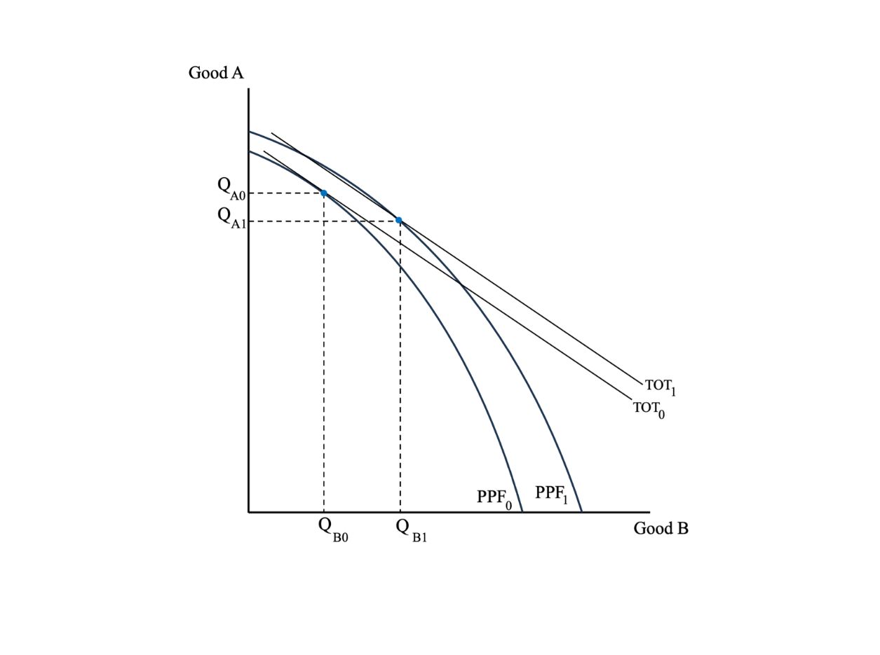
Assuming that only two products are produced in the economy and that relative product prices are constant, a country’s endowment of one factor has two effects. It raises the level of output in the sector where that factor is intensively used in production, and it lowers the level of output in the other sector. It is straightforward to see why output will expand in the sector where the factor is used intensively – greater availability of the resource makes a larger output possible. But why does output in the other sector shrink? The expanding sector not only uses the factor whose endowment has increased but also uses the other factor which did not grow. Since this other factor must be bid away from the other sector, the level of output in this sector falls. The results of the Rybczynski theorem highlight the potential for the exploitation of a new resource to restrain production in other sectors. Figure 3.6 depicts the Rybczynski theorem, whereby an increase in only one factor of production causes biased economic growth in which one sector expands at the expense of the other, assuming relative prices remain unchanged.

Economic growth also has implications for a country’s ability to trade. As we have seen, growth means that a country can produce more products and services. In addition, by raising the level of income, growth also enables a country to expand its consumption. As production and consumption change, a country’s ability to engage in international trade can change with growth, even without any change in relative product prices. Whether a country is able to trade more depends on the extent to which production and consumption change in response to economic growth.

Assuming normal goods (i.e., goods whose purchases increase with income), we can analyze a country’s ability to trade by examining the relative changes in the size of the trade triangles, which show how much a country wants to export and import. If consumption were to increase by less than production, the quantity available for export will rise. This would lead to an increase in the size of the country’s trade triangle. If consumption were to increase by more than production, the quantity available for export will decrease, and the size of the trade triangle would be smaller. The change in consumption depends on the nature of consumer preferences, depicted by the community indifference curves  (See Chapter 2). If growth is sufficiently biased in favour of the good that is initially imported, a potential drop in production in the other sector (i.e., the export sector initially) could lead to a reversal of the country’s pattern of trade. This suggests that comparative advantage can change over time.

So far, we have assumed that relative product prices have remained the same even though growth has occurred. However, economic growth can cause relative product prices (i.e., the terms of trade) to change. Changes in a country’s ability to trade can alter its terms of trade if the country is large enough for its trade volumes to affect international equilibrium product prices. To the extent that international product prices change due to trade, this affects the benefits that a country derives from economic growth. Growth can only affect international product prices if the country is able to exercise market power as a result of the volume of its exports or imports.

If economic growth results in a reduction in the price of the imported product because growth is biased toward the expansion of production in the import-competing sector, the country will benefit in two ways:

• production will increase as the production possibilities frontier shifts outward, and
• the terms of trade improve as the country now receives a higher price for its exports relative to its imports.

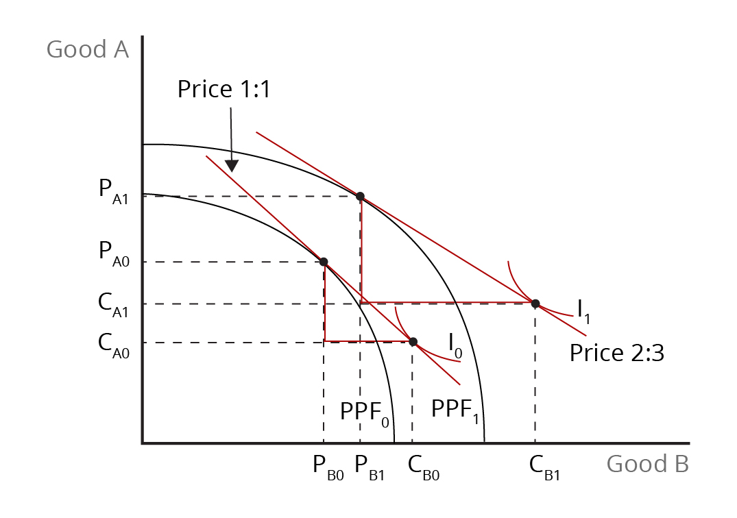
Overall, the country would be better off than it would be if relative product prices remained unchanged because it would be able to attain a higher consumption level. In addition to the gain from greater production, the country would benefit from higher relative prices. In this case, the terms of trade improvement will augment the production gain and raise the overall benefit from economic growth. Figure 3.7 shows how economic growth biased towards the import-competing sector can lead to changes in a country’s willingness to trade as well as in its international terms of trade.

It is, however, possible that growth can lead to a deterioration in the country’s terms of trade if it prompts an increase in import demand. In this case, the overall effect on the country’s well-being is not clear. It will depend on the relative strengths of the production effect and the terms of trade effect. The production effect is positive for economic well-being, but the country is negatively affected by the deterioration in the terms of trade. If the negative terms-of-trade effect is not particularly large, the country will experience an overall gain. It is possible, however, for the negative terms of trade effect to be large enough to dwarf the positive production effect.

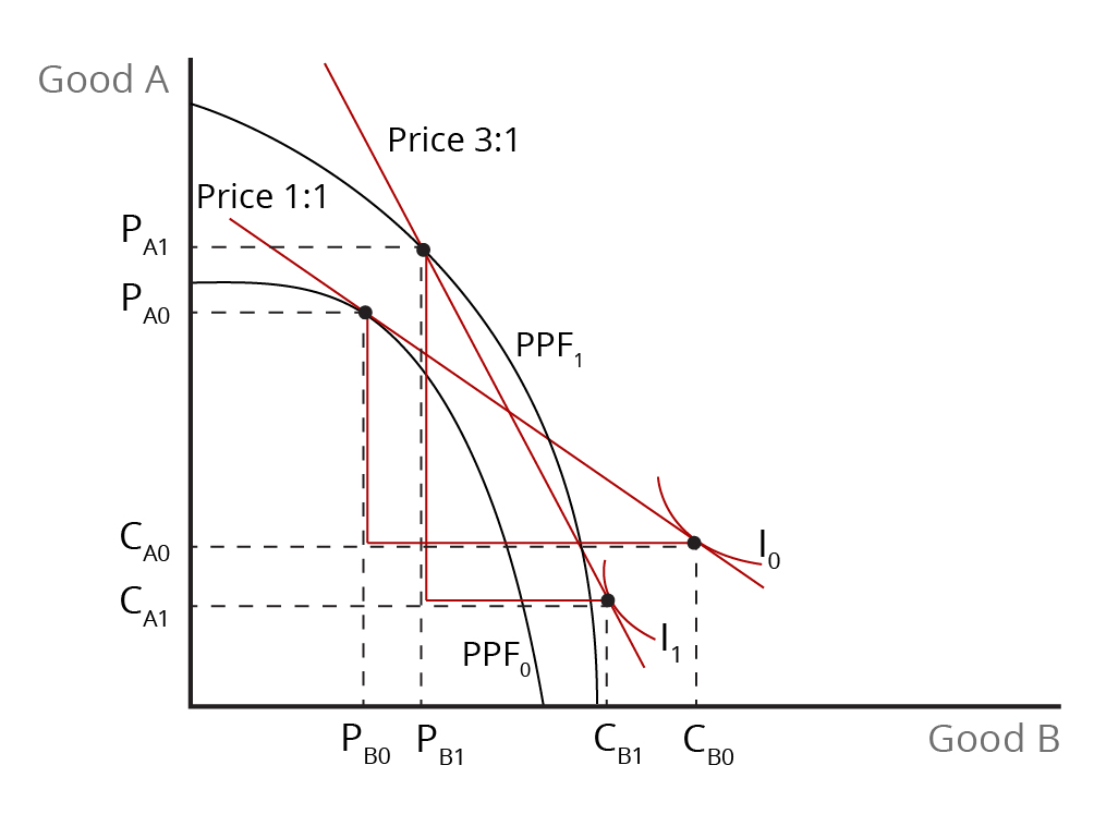
To see this, let us consider the situation in which a large country experiences a significant increase in production due to a change in technology. This lifts the economy’s output with a bias toward exports. Since the country has market power, the increase in production lowers the relative price of the export product. Graphically, the PPF shifts outward, skewed heavily toward the export sector, and the international price line steepens a lot compared with its pre-growth position (see Figure 3.8). As a result, consumption falls considerably due to the large drop in export price. Growth increases trade but prompts such a large decline in its terms of trade that the country’s economic well-being falls. This is the case of immiserizing growth, which is depicted in Figure 3.8.

References

Pugel, T. A. (2020). International economics, (17th ed.). McGraw-Hill.

Image Descriptions

Figure 3.5: Economic Growth Balanced Versus Biased

The image consists of three separate graphs, lined up horizontally, each depicting two production possibility frontiers (PPFs), labelled as PPF₀ and PPF₁, indicating different states of economic growth. Each graph represents a different type of growth.

All graphs have two axes, with the vertical axis labelled “Good A” and the horizontal axis labelled “Good B.”

• The first graph, labelled “Balanced Growth,” shows two curves that are convex to the origin, with PPF₁ lying outward from PPF0, displaying a proportional shift.
• The second graph, labelled “Biased Growth—Favours Good B,” also shows two convex curves, but here PPF₁ has pivoted clockwise slightly from PPF₀, indicating that the growth has favoured “Good B” over “Good A.”
• The third graph, labelled “Biased Growth—Favours Good A,” similarly portrays two convex curves, but with PPF₁ pivoted counter-clockwise from PPF₀, suggesting that the growth has favoured “Good A” more than “Good B.”

[back]

Figure 3.6: Illustration of the Rybczynski Theorem – Growth in a Single Factor

The image is a graph that has a vertical axis labelled “Good A” and a horizontal axis labelled “Good B.” The graph features two convex curves representing production possibility frontiers (PPFs), which intersect with two download sloping lines representing terms of trade (TOT). The lower frontier is labelled PPF₀, and the higher is labelled PPF₀. The terms of trade lines are labelled TOT₀ and TOT₁. Dashed lines project from the  PPF₀ and TOT₀ point of intersection and the PPF₁ and TOT₁ point of intersection to both axes, at “Q_A0” to “Q_A1” on the “Good A” axis and “Q_B0” to “Q_B1” on the “Good B” axis.

[back]

Figure 3.7: Growth Factoring Production in the Import Sector in a Large Country

The image is a graph with a vertical axis labelled “Good A” and a horizontal axis labelled “Good B.”

Two convex curved lines, labelled PPF₀ and PPF₁, begin two-thirds up the y-axis, and slope downward from left to right, ending in the middle of the x-axis. The PPF₁ line lies entirely above and to the right of the PPF₀ line. Four dotted horizontal lines extend from the y-axis at points P_A1, P_A0, C_A1, and C_A0, from the top down. These intersect with four dotted vertical lines extending from the x-axis, from right to left, at points P_B0, P_B1, C_B0, and C_B1.

Two points on each PPF curve are connected with red lines along the existing dotted lines at right angles. Red lines tangent to the PPFs connect through two dotted intersection points labelled Price 1:1 on PPF₀ and Price 2:3 on PPF₁. The two outer intersection points (at C_A0 and C_B0 and at C_A1 and C_B1) also have short concave lines labelled I₀ and I₁.

[back]

Figure 3.8: An Illustration of the Notion of Immiserizing Growth

The image is a graph with a vertical axis labelled “Good A” and a horizontal axis labelled “Good B.”

Two convex curved lines, labelled PPF₀ and PPF₁, begin high on the y-axis and slope downward from left to right to the middle of the x-axis. The PPF₁ line lies entirely above and to the right of the PPF₀ line. Four dotted horizontal lines extend from the y-axis at points P_A1, P_A0, C_A0, and C_A1, from the top down. These intersect with four dotted vertical lines extending from the x-axis, from right to left, at points P_B0, P_B1, C_B0, and C_B1.

Two points on each PPF curve are connected with red lines along the existing dotted lines at right angles. Red lines tangent to the PPFs connect through two dotted intersection points labelled Price 1:1 on PPF₀ and Price 3:1 on PPF₁. The two outer intersection points (at C_A1 and C_B1 and at C_A0 and C_B0) also have short concave lines labelled I₁ and I₀. The x-axis (Good B) extends beyond the graphs’ lines and points.

[back]