Lab 1: Reading landscapes from satellite imagery

Introduction

In this lab, you will practice using various tools in Google Earth to prepare you for the upcoming labs in the course. You will use the historical imagery tool to observe changes over time, take various distance and area measurements, the path tool and explore the surface of the moon and Mars. You will also practice exporting properly referenced maps from Google Earth.

To get started, ensure you have downloaded Google Earth Pro for desktop on your computer. This software is free for download from here:

https://www.google.com/earth/versions/#earthpro

Please note that although there is an online version of Google Earth, not all tools are available on the online platform. Download and open the Lab1.mkz file that contains markers for all the locations we will be visiting in this lab.

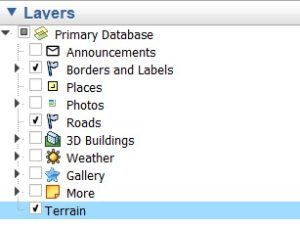
Make sure that the “Terrain” layer is selected as you complete the labs in this course, as it will allow you to see the Earth’s surface in 3D. For optimal viewing of landscapes with the least things in the way, we suggest you disable the Places, Roads, 3D Buildings, Weather, Gallery and More layers. The Photos layer can sometimes be useful for gathering on-the-ground confirmation of what a location looks like.

You can change the vertical exaggeration value of the 3D terrain. This exaggeration (set between 0.01 and 3) indicates by what factor vertical distances are exaggerated. For example, if set to 3, then vertical distances will appear 3x bigger than in real life. This can allow you to see more details, but can also cause some distortion. You can play with changing the vertical exaggeration when exploring landscapes to get a better view:

On a PC: Tools > Options > 3D View from the Tools figure
On a Mac: Google Earth > Preferences > 3D View

Tasks

1) Coordinate Formats (5 pts)

You can change the format coordinates are displayed in:

On a PC: Tools > Options > 3D View > Show lat/long
On a Mac: Google Earth > Preferences > 3D View > Show Lat/Long

You can read the coordinates of your curser as you move around the map off the bottom banner (Figure 1).

Figure 1. Example of bottom banner showing exact imagery date, coordinate, and eye altitude in Google Earth.

Fly to the Ron Joyce Field marker. Report the coordinates of the centre of the field using all the coordinate formats available in Google Earth. (5 pts)

2) Historical Imagery (7 pts)

The historical imagery tool can be accessed from the top tool bar:

Figure 2. Tool banner located at the top of the Google Earth screen with the historical imagery tool highlighted.

Once opened, you can scroll between images taken on different dates. Although the tool bar shows only the moth and year, the bar at the bottom of the window shows the exact imagery date in mm/dd/yyyy.

Scroll back in time to see how this part of campus has changed since the earliest imagery available from 1985.

a) Using the historical imagery tool determine between which dates the Ron Joyce Stadium was constructed (1 pt)

b) What was in this location before the stadium? (2 pts)

c) Look up the year the stadium was opened (1 pt)

d) Look at the Peter George Centre located next to the Ron Joyce Stadium.
Using the historical imagery tool, estimate when construction of the building began (1 pt) and finished (1 pt).

e) What was located here in 2005? (1 pt)

3) Measurements! (11 pts)

The measurement tool can be accessed from the top tool bar:

Figure 3. Tool banner located at the top of the Google Earth screen with the measurement tool highlighted.

The measurement tool allows you to measure various distances by toggling between the Line, Path, Polygon and Circle options, respectively.

a) Fly to the Ron Joyce stadium and measure the following its width (2 pts) and length between the goal posts (2 pts) in metres and yards.

b) Fly to the Parking Lot M marker. Use the path measurement tool to measure the distance between the parking lot marker and the GO bus stop on campus along the sidewalk (the path you would walk) in kilometres (1 pt). Now measure the distance between the parking lot P marker and the GO bug stop in kilometres (1 pt).

c) Use the polygon measurement tool to measure the perimeter (1 pt) and area (1 pt) of Burke Sciences Building in metres and metres squared.

d) Fly to the Mary Keyes roundabout marker on campus. Use the circle measurement tool to measure the radius of the inner edge of the road (1 pt) and the outer edge of the road (1 pt) of the roundabout. Use these values to calculate the width of the road around the roundabout (1 pt).

4) Path Tool (10 pts)

The path tool can be accessed from the top tool bar:

Figure 4. Tool banner located at the top of the Google Earth screen with the path tool highlighted.

The path tool allows you to create a permanent path layer on the map that can then be used to do additional measurements. In this lab, we will use the path tool to explore vertical profiles of paths.

a) Fly to the Parking Lot M marker. Use the path measurement tool to measure the distance between the parking lot marker and the GO bus stop on campus along the sidewalk (the path you would walk) in kilometres (1 pt). You will be able to see the path length once you create the path under the “Measurements” tab. Compare your answer to the distance you measured in question 3b and comment on why there are any discrepancies (2 pts).

b) Once you have created the path, you can see its vertical profile by right clicking on it and selecting “View elevation profile”. Using the figure that comes up, indicate whether lot M or the GO Bus stop is at a higher elevation (1 pt). Record the elevation at each of these two markers (2 pts).

c) What are these elevations relative to? (1 pt)

d) Calculate the average slope between the Lot M and Go Bus stop markers using the elevation profile figure. Show all your work (3 pts).

Remember the equation for slope:
𝑠𝑙𝑜𝑝𝑒 = 𝑐ℎ𝑎𝑛𝑔𝑒 𝑖𝑛 𝑣𝑒𝑟𝑡𝑖𝑐𝑎𝑙 (Δ𝑦) ÷ 𝑐ℎ𝑎𝑛𝑔𝑒 𝑖𝑛 ℎ𝑜𝑟𝑖𝑧𝑜𝑛𝑡𝑎𝑙 (Δ𝑥)

5) Exploring Other Worlds (5 pts)

You can toggle between exploring the Earth’s surface and that of other planetary bodies:

Figure 4. Tool banner located at the top of the Google Earth screen with the menu to toggle between views highlighted.

a) Switch to Mars view and fly to the Olympus Mons and read the information card located there. What makes this location special on the surface of Mars? (1 pt)

b) Fly to the Olympica Fossae marker and observe the strange patterns on the planet’s surface. Speculate on what might have created these features and explain your reasoning (3 pts).
Hint: Think about how similar features are created on Earth’s surface.

c) Switch to the Moon view and fly to the Apollo 13 Landing Site. What are the two named craters near the site called? (1 pt)

6) Exporting Maps (7 pts)

Return to Earth view. You will export a proper map of McMaster University campus. You can export maps as images with all the proper annotations using the Save Image tool:

Figure 5. Tool banner located at the top of the Google Earth screen with the save image tool highlighted in red. The create marker tool is highlighted in green.

Choose a building or location on campus that we have not previously explored in this lab (i.e., do NOT choose the Ron Joyce stadium, PGCLL, Parking lot M or P, the GO bus stop, or the Burke Science building). Create a marker at this building using the create marker tool and label it appropriately with the building name. Make sure all other labels and markers are unchecked, so that only your building is labelled. Export your map to create a properly exported Google Earth map of campus with your chosen building labelled and attach it to your report (1 pt). Make sure you choose a scale where the entirety of campus is visible (not just your building).

Your map should include:

• A descriptive title (1 pt)
• A north arrow (1 pt)
• NO legend (1 pt)
• A scale bar (1 pt)
• The Google logo (for referencing purposes) (1 pt)
• One building on campus labelled as a marker (no other labels should be present on the map) (1 pt)

Hint: You can toggle which elements are visible from the Map Options menu.