8.5 Inventory Models for Certain Demand: Economic Order Quantity (EOQ) Model
The Economic Order Quantity (EOQ) model is a fundamental inventory management model used when the following assumptions hold:
Assumptions
- The item is ordered from an external supplier (no internal production)
- Demand is fixed or steady over time (known with certainty)
- Lead time (the duration between order placement and receipt) is constant
- A fixed order quantity is placed each time
- The ordering cost is fixed per order, regardless of order size
Inventory Control Cycles
Each order placement initiates an inventory control cycle or order cycle. Upon receiving an order, the inventory level increases, and as demand is satisfied, the inventory level decreases over time. When the inventory level reaches a predetermined reorder point, a new order is placed, and the cycle repeats.
The inventory level fluctuates, as shown in the following diagram:
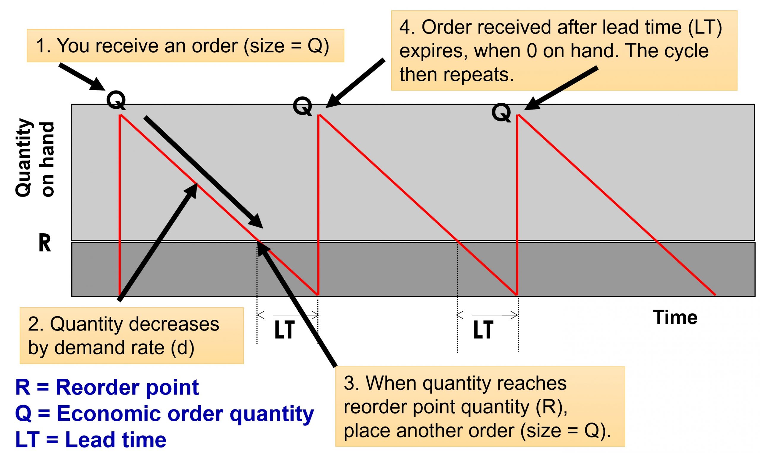
At point 1, an order of quantity Q is received, increasing the inventory level from zero to Q units. As time progresses, the inventory level decreases due to demand. When the inventory level reaches the reorder point R, a new order is placed to ensure that the order is received just as the inventory level reaches zero, preventing stock-outs.
Objective and Cost Components
The objective of the EOQ model is to determine the optimal order quantity (Q*) that minimizes the total relevant costs, which include:
- Total Ordering Costs
- Total Inventory Holding (Carrying) Costs
Other costs, such as total acquisition (purchasing) costs and shortage costs, are excluded from the model due to the assumptions of fixed demand and no stock-outs.
Notation and Calculations
Let:
D = demand (units/year)
Q = order quantity
S = order cost ($/order)
H = carrying cost ($/item/year)
Iavg = Average inventory
N = number of orders per year
TC = Total Cost
Total Cost = Ordering cost + Carrying cost
TC = ( S × N ) + (H × Iavg)
TC(Q) = ( S × D ÷ Q ) + ( H × Q ÷ 2 )
The number of orders per year (N) can be calculated as N = D÷Q.
The average inventory level is Q÷2, assuming a constant demand rate.
The total relevant cost function, TC(Q), is given by:
[latex]TC(Q)\;=\;(D\div Q)\;\times\;S\;+\;(Q\div2)\;\times\;H[/latex]
By setting the derivative of TC(Q) with respect to Q equal to zero and solving for Q, the optimal order quantity Q* is obtained:
[latex]Q^\ast=\sqrt{\frac{2DS}H}[/latex]
This optimal order quantity minimizes the total relevant costs for the given demand, ordering cost, and holding cost parameters.
The EOQ model provides a straightforward approach to determining the optimal order quantity when demand is certain, and other assumptions are met, enabling organizations to optimize their inventory management strategies and minimize associated costs.
The * on top of Q shows that it is a special value of the Q, which, in this case, is the optimal value. Let’s have a look at some examples.
Video: "Inventory Management: Economic Order Quantity (EOQ) Model Video 1" by Excel@Analytics - Dr. Canbolat [15:25] is licensed under the Standard YouTube License.Transcript and closed captions available on YouTube.
Examples
Example 1
Assume that Apple Canada has an annual demand of 250,000 for one of its tablets. A component has annual holding cost of $12 per unit, and ordering cost of $150. Calculate EOQ, total cost of ordering and inventory holding, number of orders per year and the order cycle time for this item. Assume 250 working days in a year.
Solution
H = $12 per unit
S = $150
D = 250,000 units
[latex]EOQ=Q^\ast=\sqrt{\frac{2DS}H}=\sqrt{\frac{2\times250,000\times150}{12}}=2500[/latex]
[latex]TC(Q^\ast)=S\times\frac D{Q^\ast}+H\times\frac{Q\ast}2=150\times\frac{250,000}{2500}+12\times\frac{2500}2=15000+15000=\$30,000[/latex]
[latex]\text{Optimal number of orders per year }=\frac D{Q^\ast}=\frac{250,000}{2500}=100[/latex]
[latex]\text{Length of order cycle time }=\frac{250\;\text{days in a year}}{100\;\text{orders}}=2.5\;\text{days}[/latex]
Example 2
Assume that it costs BestBuy $625 each time it places an order with a manufacturer for a specific model of laptop. The cost of carrying one laptop in inventory for a year is $130. The store manager estimates that total annual demand for the laptops will be 1500 units, with a constant demand rate throughout the year. The store policy is never to have stockouts of the laptops. The store is open for business every day of the year except Christmas Day.
Determine the following:
- Optimal order quantity per order
- Minimum total annual inventory costs
- The optimal number of orders per year
- The time between orders (in working days)
Solution
D = 1500
S = $625
H = $130
a. [latex]Q\ast=\sqrt{\frac{2DS}H}=\sqrt{\frac{2(1500)(625)}{130}}=120.1[/latex]
b. [latex]TC(Q)=\frac{SD}Q+\frac{HQ}2=\frac{625\times1500}{120.1}+\frac{130\times120.1}2=\$15,612.49[/latex]
c. [latex]\frac DQ=\frac{1500}{120.1}=12.49\;\text{orders}[/latex]
d. [latex]\frac{364}{12.49}=29.14\;\text{days}[/latex]
Example 3
The Modern Furniture Company purchases upholstery material from textile supplier in Halifax, Canada. The company uses 45,000 yards of material per year to make sofas. The cost of ordering material from the textile company is $1500 per order. It costs Modern Furniture $0.70 per yard annually to hold a yard of material in inventory. Determine:
- The optimal number of yards of material Modern Furniture should order
- The minimum total inventory cost
- The optimal number of orders per year, and
- The optimal time between orders
Solution
D = 45,000
S = $1500
H = $0.70
a. [latex]Q\ast=\sqrt{\frac{2DS}H}=\sqrt{\frac{2(45000)(1500)}{0.70}}=13,887.3\;\text{yd}[/latex]
b. [latex]TC(Q)=\frac{SD}Q+\frac{HQ}2=\frac{1500\times45000}{13887.3}+\frac{0.7\times13887.3}2=\$9721.11[/latex]
c. [latex]\frac DQ=\frac{45000}{13887.3}=3.24\;\text{orders per year}[/latex]
d. [latex]\frac{365}{3.24}=112.6\;\text{days}[/latex]
“Inventory Management” from Introduction to Operations Management Copyright © by Hamid Faramarzi and Mary Drane is licensed under a Creative Commons Attribution-NonCommercial-ShareAlike 4.0 International License, except where otherwise noted.—Modifications: used section Inventory Models for Certain Demand: Economic Order Quantity (EOQ), some paragraphs rewritten or in some cases removed; added additional explanations; video added.
