3.7 Time Series Models
Time series data plays a fundamental role in forecasting. A time series collects data points meticulously ordered along a time axis. These data points can be recorded at consistent or irregular intervals. Examples of time series data include ocean tide heights, sunspot counts, and daily closing values of stock market indices. Line charts are a prevalent method for visualizing time series data.
Excel offers a forecast function that can be used for forecasting. The following video shows how it is done.
Video: "The Excel FORECAST Function" by Technology for Teachers and Students [5:31] is licensed under the Standard YouTube License.Transcript and closed captions available on YouTube.
The application of time series analysis extends across numerous disciplines, including statistics, signal processing, pattern recognition, econometrics, mathematical finance, weather forecasting, earthquake prediction, and various domains of applied science and engineering that involve temporal measurements. By leveraging time series data, these fields can uncover hidden patterns, trends, and seasonality within the data, enabling the formulation of data-driven forecasts for future outcomes (Singla, 2018).
Selecting the Appropriate Time Interval for Data Collection
A critical aspect of forecasting accuracy lies in determining the optimal time interval for data collection. The chosen interval directly impacts the level of data fluctuation observed. This fluctuation can manifest as trends, seasonal patterns, cyclical variations, or random noise. Understanding the specific fluctuation behaviour of the data is instrumental in selecting the most suitable forecasting technique.
It's important to remember that time intervals are inherently relative. Terms like "short-term," "medium-term," and "long-term" are context-dependent. Table 3.7.1 overviews various forecasting techniques, categorized based on their typical time horizons. Generally, short-term forecasts involve data collected over less than three months, while medium-term forecasts encompass three months to 2 years. Long-term forecasts, however, deal with data collected over a timeframe exceeding two years.
| Time Period | Data Pattern | Forecasting Technique |
|---|---|---|
| Short term: less than 3 months | Data does not show any particular pattern or variation |
|
| Medium-term: 3 months to two years | Data either repeats periodically or moves in a particular direction, i.e. upward or downward. |
|
| Long-term: more than 2 years | Data shows a repeated pattern but at irregular intervals with irregular intensity. |
|
Time Period Selection and Forecast Accuracy
The chosen time period for data collection plays a crucial role in forecast accuracy. While a longer timeframe may intuitively suggest more reliable results, older data may lose relevance in the present context. Conversely, relying solely on recent data might not provide a sufficient historical foundation for generating dependable forecasts. This highlights the importance of striking a balance between the time period selected and the availability of relevant data within that timeframe. Ultimately, the optimal time horizon depends on the specific forecasting problem and the nature of the data itself.
Trend Analysis
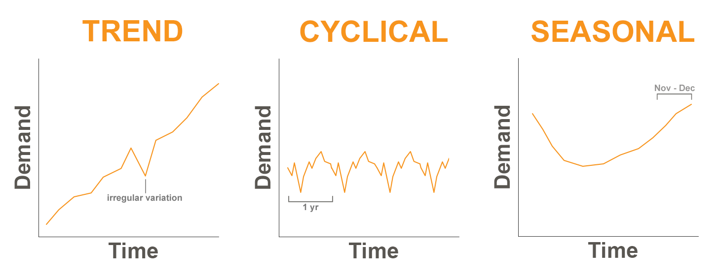
When we plot our historical product demand, the following patterns can often be found:
- Trend – This component represents a consistent upward or downward movement in the data over time. The product life cycle often plays a role in shaping this trend. A new product might exhibit a rising sales trend, while a mature product might show a declining trend.
- Cyclical – Cyclical patterns are characterized by recurring fluctuations in the data that typically span more than a year. These cycles can be linked to factors like interest rates, political climates, consumer confidence, or broader market dynamics.
- Seasonal – Many products exhibit seasonal patterns, featuring predictable changes in demand that recur annually. Fashion apparel and sporting goods are prime examples of products significantly impacted by seasonality. Demand for winter coats surges during the cold season, while swimwear sales peak during summer.
- Irregular variations – Unforeseen events or series of events can influence demand in unpredictable ways. These irregular variations, often referred to as outliers, are not expected to be repeated in the future. Examples include extreme weather events, labour strikes, or power outages. These events can cause sudden spikes or dips in demand data.
- Random variations – Random variations, also referred to as noise, represent the unexplained fluctuations in demand that persist even after accounting for all other identifiable components. These variations are inherent in any time series data and cannot be attributed to any specific cause.
Naïve Method
The naive approach, also known as naive forecasting or naïve method, is one of the simplest forecasting techniques used in operations management. It involves using the actual value from the previous period as the forecast for the next period without considering any other factors or patterns in the data.
The naive approach is based on the assumption that the future value of a variable will be the same as its most recent observed value. Its characteristics include simplicity, no trend or seasonality consideration, and limited data requirements. (What do you need to know about naïve forecasting?, 2024)
|
Advantages |
Disadvantages |
|---|---|
|
Easy to implement |
Ignores patterns and trends |
|
It can serve as a baseline or benchmark for comparison |
Unsuitable for new products/services |
|
Suitable for stable demand |
Reactive rather than proactive |
Simple Moving Average
The simple moving average method is fundamental for forecasting future values based on historical data. It operates by calculating the average of the data points from the most recent n periods. The selection of the appropriate value for n is crucial and can be influenced by various factors, such as the underlying data characteristics and the desired forecast accuracy. For instance, a manager might leverage demand data from the past four periods (n = 4) to generate a 4-period moving average forecast for the upcoming period.
This method is advantageous due to its simplicity and ease of computation. However, it also has limitations. By assigning equal weight to all data points within the window, it may not adequately capture recent trends or sudden shifts in the data. More sophisticated moving average methods address this limitation by incorporating weights that prioritize the most recent data points, placing greater emphasis on their influence on the forecast.
Example
Some relevant notation:
Dt = Actual demand observed in period t
Ft = Forecast for period t
Using the following table, calculate the forecast for period 5 based on a 3-period moving average.
|
Period |
Actual Demand |
|---|---|
|
1 |
42 |
|
2 |
37 |
|
3 |
34 |
|
4 |
40 |
Solution
Forecast for period 5 = F5 = (D4 + D3 + D2) ÷ 3 = (40 + 34 + 37) ÷ 3 = 111 ÷ 3 = 37
Weighted Moving Average
This method is the same as the simple moving average with the addition of a weight for each one of the last “n” periods. In practice, these weights need to be determined in a way to produce the most accurate forecast. Let’s have a look at the same example, but this time, with weights:
Example
|
Period |
Actual Demand |
Weight |
|---|---|---|
|
1 |
42 |
|
|
2 |
37 |
0.2 |
|
3 |
34 |
0.3 |
|
4 |
40 |
0.5 |
Solution
Forecast for period 5 = F5 = (0.5 × D4 + 0.3 × D3 + 0.2 × D2) = (0.5 × 40 + 0.3 × 34 + 0.2 × 37) = 37.6
Note that if the sum of all the weights were not equal to 1, this number above had to be divided by the sum of all the weights to get the correct weighted moving average.
Exponential Smoothing
The exponential smoothing method integrates the most recent actual demand and the previous forecast to generate the forecast for the upcoming period. This approach offers several advantages. Firstly, it often yields more accurate forecasts. Secondly, it is a straightforward method that enables forecasts to adapt to new trends or changes in demand patterns swiftly. A notable benefit of exponential smoothing is that it does not necessitate a large volume of historical data.
Exponential smoothing employs a smoothing coefficient, denoted as Alpha (α). The value of Alpha determines the rate at which the forecast responds to fluctuations in demand. Consequently, Alpha is also referred to as the Smoothing Factor. A higher value of Alpha implies that the forecast will react more rapidly to changes in demand, while a lower value will result in a more gradual response, effectively smoothing out the fluctuations.
In essence, the exponential smoothing method balances the most recent demand observation and the previous forecast, with the smoothing coefficient Alpha governing the relative weights assigned to each component. This approach enables the forecast to adapt to evolving demand patterns while mitigating the impact of random fluctuations, thereby enhancing forecast accuracy and responsiveness.
There are two versions of the same formula for calculating the exponential smoothing.
Version #1:
[latex]F_{t\;}=\;(1\;\;-\;\alpha)\;F_{t-1}+\;\alpha\;D_{t-1}[/latex]
Note that α is a coefficient between 0 and 1
For this method to work, we need to have the forecast for the previous period. This forecast is assumed to be obtained using the same exponential smoothing method. If there were no previous period forecasts for any of the past periods, we would need to initiate this method of forecasting by making some assumptions. This is explained in the next example.
Example
|
Period |
Actual Demand |
Forecast |
|---|---|---|
|
1 |
42 |
|
|
2 |
37 |
|
|
3 |
34 |
|
|
4 |
40 |
|
|
5 |
|
|
In this example, period 5 is the next period for which we are looking for a forecast. In order to have that, we will need the forecast for the last period (i.e., period 4). But there is no forecast given for period 4. Thus, we will need to calculate the forecast for period four first. However, a similar issue exists for period four since we do not have the forecast for period 3. So, we need to go back for one more period and calculate the forecast for period 3. As you see, this will take us all the way back to period 1. Because there is no period before period 1, we will need to make some assumptions for the forecast of period 1. One common assumption is to use the same demand of period 1 for its forecast. This will give us a forecast to start, and then we can calculate the forecast for period two from there. Let’s see how the calculations work out:
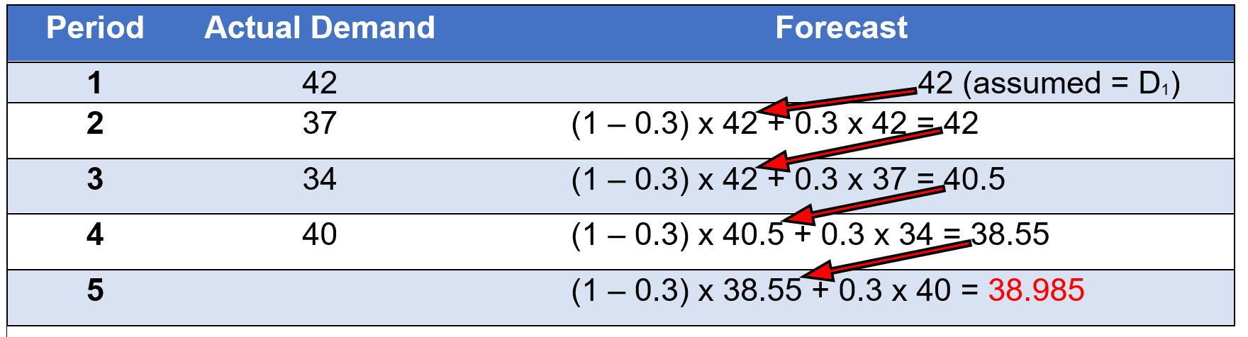
If α = 0.3 (assume it is given here, but in practice, this value needs to be selected properly to produce the most accurate forecast)
Assume F1 = D1, which is equal to 42.
Then, calculate F2 = (1 − α) F1 + α D1 = (1 − 0.3) × 42 + 0.3 × 42 = 42
Next, calculate F3 = (1 − α) F2+ α D2 = (1 − 0.3) × 42 + 0.3 × 37 = 40.5
And similarly, F4 = (1 − α) F3+ α D3 = (1 − 0.3) × 40.5 + 0.3 × 34 = 38.55
And finally, F5 = (1 − α) F4+ α D4 = (1 − 0.3) × 38.55 + 0.3 × 40 = 38.985
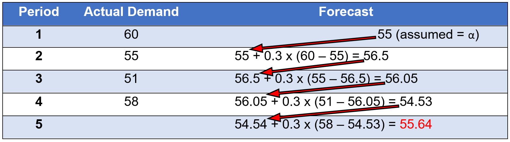
Version #2:
[latex]F_{t\;}=\;F_{t-1}+\;\alpha\;(D_{t-1}-F_{t-1})[/latex]
Example
Assume you are given an alpha of 0.3
Seasonal Index
A seasonal index is a statistical tool used in forecasting to quantify and account for recurring seasonal patterns or demand fluctuations over a specific period.
It helps to identify and measure the impact of seasonal factors (e.g. holidays, weather, etc.) on demand for a product or service so that the organizations adjust forecasts to account for predictable seasonal variations.
The seasonal index is calculated by comparing demand during a specific season/period to the average demand across all seasons/periods. It is typically calculated as a ratio or percentage, with an index value above one indicating higher than average demand and below 1 indicating lower demand.
Historical demand data is deseasonalized by dividing it by the respective seasonal index to remove seasonal effects. Forecasting methods like moving averages or exponential smoothing are applied to the deseasonalized data. The resulting forecast is then re-seasonalized by multiplying it with the appropriate seasonal indexes.
Seasonal indexing is useful for products/services with recurring seasonal demand patterns like holidays, back-to-school, weather changes, etc. It helps to plan inventory levels, staffing, promotions, and other operations aligned with expected seasonal fluctuations (Singla, 2018).
Example
|
Season |
Previous Sales |
Average Sales |
Seasonal Index |
|---|---|---|---|
|
Winter |
390 |
500 |
390 ÷ 500 = .78 |
|
Spring |
460 |
500 |
460 ÷ 500 = .92 |
|
Summer |
600 |
500 |
600 ÷ 500 = 1.2 |
|
Fall |
550 |
500 |
550 ÷ 500 = 1.1 |
|
Total |
2000 |
|
|
Using these calculated indices, we can forecast the demand for next year based on the expected annual demand for the next year. Let’s say a firm has estimated that next year's annual demand will be 2500 units.
|
Season |
Anticipated annual demand |
Avg. Sales ÷ Season |
Seasonal Factor |
New Forecast |
|---|---|---|---|---|
|
Winter |
|
625 |
0.78 |
.78 × 625 = 487.5 |
|
Spring |
|
625 |
0.92 |
.92 × 625 = 575 |
|
Summer |
|
625 |
1.2 |
1.2 × 625 = 750 |
|
Fall |
|
625 |
1.1 |
1.1 × 625 = 687.5 |
|
|
2500 |
|
|
|
"3 Forecasting" from Introduction to Operations Management Copyright © by Hamid Faramarzi and Mary Drane is licensed under a Creative Commons Attribution-NonCommercial-ShareAlike 4.0 International License, except where otherwise noted. Modifications: added section on - Selecting the Appropriate Time Interval for Data Collection
"Time Series Methods of Forecasting" in Operations Management by Vikas Singla, licensed under a Creative Commons Attribution-NonCommercial 4.0 International License, except where otherwise noted.
